Chapter 7 - Left Truncation and Interval Censoring

Slides

Lecture slides here. (To convert html to pdf, press E \(\to\) Print \(\to\) Destination: Save to pdf)

Base R Code

Show the code

##################################################################
# This code generates all numerical results in chapter 7.      ##
##################################################################

library(survival)

# read in the Channing study data
channing <- read.table("Data\\Channing House Study\\channing.txt")

head(channing)

# fit a Cox model to the Channing study data
# with entry age as left-truncation time
obj <- coxph(Surv(Entry.Age, End.Age, status) ~ factor(gender), data=channing)

summary(obj)

### proportionality of gender ####
# Schoenfeld residuals
obj_zph <- cox.zph(obj)
# test result
obj_zph
# plot the rescaled residuals
plot(obj_zph, ylab = "Gender", xlab = "Age (years)", lwd = 2)

### prediction of (conditional survival) ##

library(tidyverse)
## numbers at risk
t <- seq(60, 100, by = 1)

## function to compute number at risk
## at each t based on entry (T_L) and end (X)
n_risk_t <- function(entry, end){
  m <- length(t)
  n_j <- rep(NA, m)
  for (j in 1:m){
    n_j[j] <- sum(entry <= t[j] & t[j] <= end)
  }
  return(n_j)
}

## compute n at risk by gender
nrisk<- channing |> 
  group_by(gender) |> 
  reframe(
    n_j = n_risk_t(Entry.Age, End.Age)
  ) |> 
  add_column(
    t = rep(t, 2),
    .before = 1
  ) |> 
  mutate(
    gender = if_else(gender == 1, "Male", "Female")
  )

# plot n at risk by gender
nrisk_fig <- nrisk |> 
  ggplot(aes(x = t, y = n_j)) +
  geom_step(aes(linetype = gender)) +
  theme_bw() +
 labs(
   x = "Age (years)",
   y = "Number at risk"
 ) +
 theme(
    legend.title = element_blank(),
    legend.position = "top"
  )

# set cut-off 70 yo
t0 <- 70
# get model-based parameter estimates
beta <- obj$coefficients
Lambda0 <- basehaz(obj, centered = FALSE)
Lambda0t0 <- Lambda0[Lambda0$time >= t0,]
Lambda0t0$hazard <- Lambda0t0$hazard - Lambda0t0$hazard[1] ## conditional cum hazard after t0


# predicted gender-specific conditional 
# survival functions given 70 yo
surv_t0 <- Lambda0t0 |> 
  mutate(
    St = exp(- hazard),
    gender = "Male"
  ) |> 
  add_row(
    Lambda0t0 |> 
      mutate(
        St = exp(- hazard * exp(beta)),
        gender = "Female"
      )
  )

# plot conditional survival functions
surv_fig <- surv_t0 |> 
  ggplot(aes(x = time, y = St)) +
  geom_step(aes(linetype = gender)) +
  theme_bw() +
  labs(
    x = "Age (years)",
    y = "Conditional survival probabilities"
  ) +
  theme(
    legend.title = element_blank(),
    legend.position = "top"
  ) +
  scale_x_continuous(expand = expansion(c(0, 0.05)))

## package to combine plots
library(patchwork)
# combine n-at-risk and conditional-survival plots
chan_model <- nrisk_fig + surv_fig + plot_layout(ncol = 2, guides = "collect") & 
  theme(legend.position = 'top')

# ggsave("trunc_chan_model.pdf", chan_model, width = 8, height = 4)
# ggsave("trunc_chan_model.eps", chan_model, width = 8, height = 4)



## BMA HIV study
## Bangkok Metropolitan Administration HIV Study
data <- read.table("Data//Bangkok Metropolitan Administration HIV_AIDS Study//bam.txt")


# install the IntCens package from local file
install.packages("IntCens_0.1.0.tar.gz",
                 repos = NULL,
                 type = "source")
library(IntCens)

## BMA data
head(data)

# get the response data for ICSurvICM()
delta <- data$delta
gamma <- data$gamma
n <- nrow(data)
U <- data$U
V <- data$V


# Fit a proportional hazards model
obj.PH <- ICSurvICM(delta,gamma,U,V,Z = data[,5:9],model="PH")
print.ICSurv(obj.PH)


# obj.PO <- ICSurvICM(delta,gamma,U,V,Z=data[,5:9],model="PO")


# Table 7.3
# construct a table for hazard ratio and
# 95% confidence intervals

#regression parameter
beta <- obj.PH$beta
se <- sqrt(diag(obj.PH$var))
c1 <- round(exp(beta),2)
c2 <- paste0("(",round(exp(beta-1.96*se),2),", ",
   round(exp(beta+1.96*se),2),")")
noquote(cbind(c1,c2))



# Prediction of HIV sero-negative probabilities for a median-aged male IDU
# without histories of needle sharing or drug injection in jail by prior imprisonment
# status.
par(mfrow=c(1,1))
age.med <- median(data[,"age"])
plot.ICSurv(obj.PH, z=c(age.med,1,0,0,0),xlim=c(0,50), lty = 2,
     xlab="Time (months)",ylab="HIV sero-negative probabilities",
     lwd=2, main = "")
plot.ICSurv(obj.PH, z=c(age.med,1,0,1,0), xlim=c(0,50), add=T,
     lwd=2)
legend(0, 0.3, lty=c(2, 1), c("Not jailed before","Jailed before"), lwd=2)

Follow-up Plots

Visualization of subject-level follow-up under left truncation or interval censoring must account for the nonzero entry time or the imprecise location of the endpoint. This makes it different from right-censored data. To show the additional information, we need additional features on the plot.

Under left truncation

For each subject, we use a line segment to represent the period \([T_{Li}, X_i]\) on study, at the end of which the outcome event is distinguished from censoring by point shape.

The following is an example using the Channing House study.

library(tidyverse)
# read in the Channing study data
channing <- read.table("Data\\Channing House Study\\channing.txt")

# head(channing)
# take a random sample of 100 females
set.seed(2024)
channing_f_sub <- channing |> 
  filter(gender == 2) |> 
  sample_n(100)
# take all males
channing_m_sub <- channing |> 
  filter(gender == 1) 

# combine the sub-samples
channing_sub <- channing_f_sub |> add_row(channing_m_sub)
n <- nrow(channing_sub) # number of subjects in the sub-sample

# panel labeller
gender_labeller <- c("1" = "Males", "2" = "Females")

# follow -up plot
chan_fig <- channing_sub |> 
  add_column(ID = 1 : n) |> # add an ID column as y-axis
  ggplot(aes(y = reorder(ID, End.Age))) + # order subject ID shown on y-axis by end time
  geom_linerange(aes(xmin = Entry.Age, xmax = End.Age)) + # line range (T_L, X)
  geom_point(aes(x = Entry.Age, shape = "2"), fill = "white", size = 2) + # entry point (2)
  geom_point(aes(x = End.Age, shape = factor(status)), fill = "white", size = 2)  + 
  # endpoint (1: event; 0: censoring)
  geom_vline(xintercept = 60, linewidth = 1) + # start line at age 60
  facet_wrap(~ gender, ncol = 2, scales = "free", # by gender
             labeller = labeller(gender = gender_labeller)) +
  theme_minimal() +
  scale_y_discrete(name = "Subjects") +
  scale_x_continuous(name = "Age (years)", limits = c(60, 100), 
                     breaks = seq(60, 100, by = 10), 
                     expand = expansion(c(0, 0.05)))  +
  scale_shape_manual(limits = c("2", "0", "1"),  values = c(22, 23, 19), 
                      labels = c("Admission", "Censoring", "Death")) + # set the point shapes
  theme( # theme formatting
    legend.position = "top",
    legend.title = element_blank(),
    axis.text.y = element_blank(),
    axis.ticks.y = element_blank(),
    panel.grid.major.y = element_blank(),
    legend.text = element_text(size = 11),
    axis.title = element_text(size = 11),
    axis.text = element_text(size = 10),
    strip.text = element_text(size = 10)
  )

chan_fig
# ggsave("trunc_chan_fig.pdf", chan_fig, width = 8, height = 9)
# ggsave("trunc_chan_fig.eps", chan_fig, width = 8, height = 9)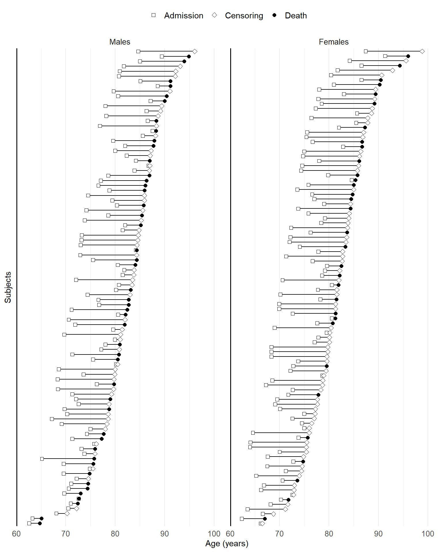

Figure 1: Follow-up plots for a random sample of 100 residents for each gender in the Channing House study. Males appear to suffer more deaths than females.

Under interval censoring

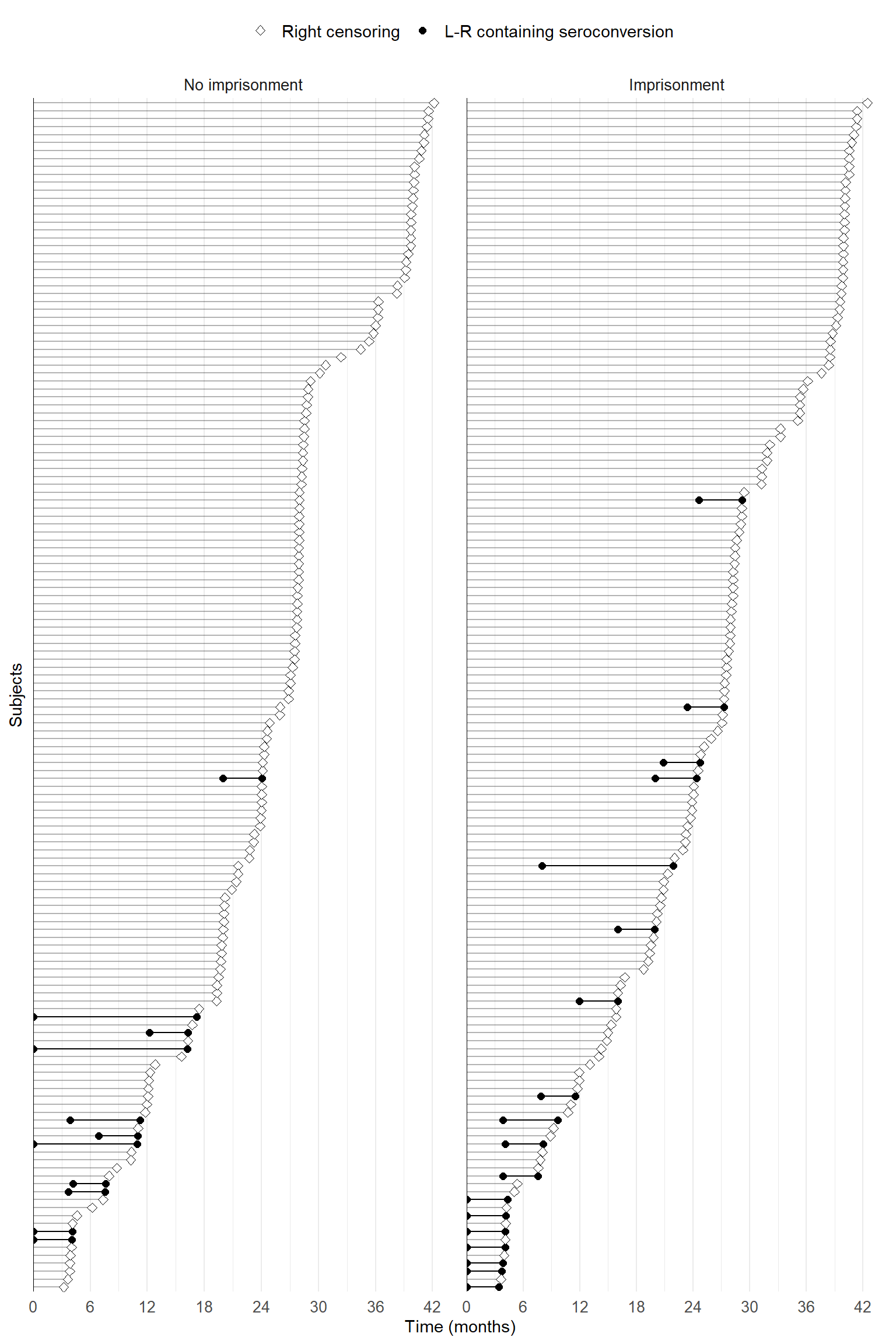
For each subject, we use a gray line to represent the follow-up period. The check-up times can be marked on it by dots if such data are available. The event-containing interval \([L_i, R_i]\) (\(R_i<\infty\)) is highlighted from the rest of the follow-up period using a black line segment.

The following is an example using the Bangkok Metropolitan Administration HIV study.

library(IntCens)
## BMA HIV study
## Bangkok Metropolitan Administration HIV Study
bma <- read.table("Data//Bangkok Metropolitan Administration HIV_AIDS Study//bam.txt")

# sample size
n <- nrow(bma)

# create L and R
bma_lr <- bma |> 
  mutate(
    ID = 1 : n, 
    L = case_when(
      delta == 1 ~ 0,
      gamma == 1 ~ U,
      delta + gamma == 0 ~ V
    ),
    R = case_when(
      delta == 1 ~ U,
      gamma == 1 ~ V,
      delta + gamma == 0 ~ Inf
    ),
    .before = 1
  )

# take a random sample of 150 subjects per imprisonment status
set.seed(2024229)
bma_lr_jail_sub <- bma_lr |> 
  filter(jail == 1) |> 
  sample_n(150) 
  
bma_lr_nojail_sub <- bma_lr |> 
  filter(jail == 0) |> 
  sample_n(150) 

## combine the sub-samples
bma_lr_sub <- bma_lr_jail_sub |> 
  add_row(bma_lr_nojail_sub) |> 
  mutate(
    end = ifelse(R == Inf, L, R),
    status = (R < Inf) + 0 # an indicator of event occurence vs right censoring
  )


# panel labeller
jail_labeller <- c("0" = "No imprisonment", "1" = "Imprisonment")

# follow -up plot
bma_fig <- bma_lr_sub |> 
  ggplot(aes(y = reorder(factor(ID), end))) + # order subjects by R or last check-up
  geom_linerange(aes(xmin = 0, xmax = L), alpha = 0.3) + # gray line for non-event-containing period
  geom_linerange(data = bma_lr_sub |> filter(status == 1), 
    aes(xmin = L, xmax = R), linetype = 1) + # black line for event-containing interval
  geom_point(data = bma_lr_sub |> filter(status == 1), aes(x = L, shape = "1"), size = 2) +
  geom_point(data = bma_lr_sub |> filter(status == 1), aes(x = R, shape = "1"), size = 2) +
  geom_point(data = bma_lr_sub |> filter(status == 0), aes(x = L, shape = "0"), 
             fill = "white", size = 2) + # different point shapes
  geom_vline(xintercept = 0) +
  facet_wrap(~ jail, scales = "free", labeller = labeller(jail = jail_labeller)) + 
  # by imprisonment status
  theme_minimal() +
  scale_y_discrete(name = "Subjects") +
  scale_x_continuous(name = "Time (months)", 
                     breaks = seq(0, 48, by = 6), 
                     expand = expansion(c(0, 0.05))) +
  scale_shape_manual(limits = c("0", "1"),  values = c(23, 19), 
                      labels = c("Right censoring", "L-R containing seroconversion")) +
  # set point shapes
 theme( # theme formatting
    legend.position = "top",
    legend.title = element_blank(),
    axis.text.y = element_blank(),
    axis.ticks.y = element_blank(),
    panel.grid.major.y = element_blank(),
    legend.text = element_text(size = 11),
    axis.title = element_text(size = 11),
    axis.text = element_text(size = 10),
    strip.text = element_text(size = 10)
  )

bma_fig
# ggsave("trunc_bma_fig.pdf", bma_fig, width = 8, height = 12)
# ggsave("trunc_bma_fig.eps", bma_fig, width = 8, height = 12, device = cairo_pdf)

Figure 2: Follow-up plots for a random sample of 150 intravenous drug users by imprisonment history in the Bangkok Metropolitan Administration study. Those who have been imprisoned before appear more likely to experience sero-conversion.