library(survival)
# Example data frame 'mydata' with columns:
#   time: Event or censoring time
#   status: Event indicator (1 if event observed, 0 if censored)
#   x1, x2: Covariates
#   group: A grouping variable (e.g., for stratification)

# 1. Fit a basic Cox model
obj <- coxph(Surv(time, status) ~ x1 + x2, data = mydata)

# 2. Summarize the fitted model
summary(obj)
# This provides coefficient estimates (log-hazard), hazard ratios (exp(coef)),
# standard errors, confidence intervals, and p-values.

# 3. Obtain Breslow estimates of the baseline cumulative hazard
base_haz <- basehaz(obj, centered = FALSE)
head(base_haz)

# 4. Extract residuals for diagnostics
mart_res <- residuals(obj, type = "martingale")   # Martingale residuals
sch   <- cox.zph(obj)   # Schoenfeld residuals and tests

# 5. Fit a stratified Cox model
obj_str <- coxph(Surv(time, status) ~ x1 + x2 + strata(group), data = mydata)

# 6. Fit a Cox model with time-varying covariates
# (Requires data in long "start-stop" format)
obj_tv <- coxph(Surv(start, stop, event) ~ x1 + tv_cov, data = tv_data)Chapter 4 - Cox Proportional Hazards Regression
\[ \def\T{\mathrm{T}} \]
Slides
Lecture slides here. (To convert html to pdf, press E \(\to\) Print \(\to\) Destination: Save to pdf)
Chapter Summary
The Cox proportional hazards model is a most popular semiparametric regression model for time-to-event data. The partial likelihood provides a key tool for making inferences on parametric covariate effects in the presence of a nonparametric time trend.
Basic model specification
The Cox proportional hazards model expresses each subject’s hazard rate as a product of a baseline function and an exponential term involving covariates. For a subject with covariates \(Z\), the hazard at time \(t\) is
\[ \lambda(t \mid Z) = \lambda_0(t)\exp(\beta^{\rm T} Z). \]
This decomposition leaves \(\lambda_0(t)\) fully unspecified, focusing on the log-hazard coefficients \(\beta\). Under proportional hazards, any two covariate sets differ by a constant hazard ratio over time, enabling a direct interpretation of \(\exp(\beta_k)\) as the risk multiplier per unit increase in the \(k\)-th covariate.
The partial-likelihood approach
Estimation of \(\beta\) proceeds through a partial-likelihood function that isolates each event’s contribution while conditioning on the subjects at risk. Suppose the observed sample has unique failure times \(t_1 < \dots < t_m\), each with a single failing subject denoted by \((j)\). Let \(\mathcal{R}_j\) be the risk set at \(t_j\), meaning the indices of all subjects still under observation just before \(t_j\).
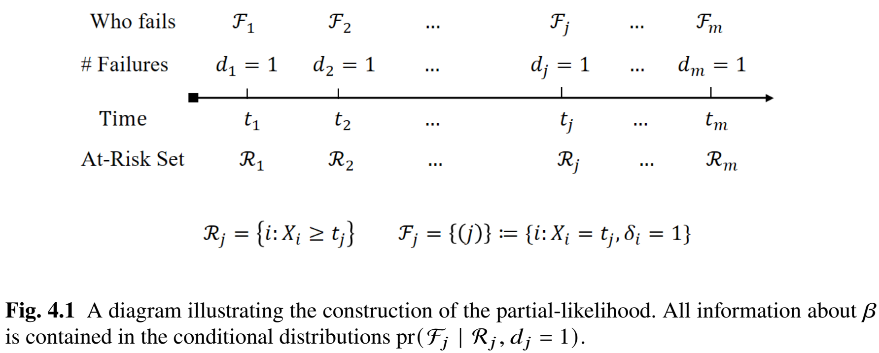
Then the Cox partial likelihood is
\[ PL(\beta) = \prod_{j=1}^m \frac{ \exp(\beta^\T Z_{(j)}) }{ \sum_{i \in \mathcal{R}_j} \exp(\beta^\T Z_i) }, \] where \(Z_{(j)}\) is the covariate vector for the subject who fails at \(t_j\). This construction eliminates \(\lambda_0(t)\) from the likelihood by focusing on how the failures are “allocated” among those at risk.
Taking logarithms leads to the log-partial likelihood,
\[ \log PL(\beta) = \sum_{j=1}^m \left[ \beta^\T Z_{(j)} \;-\; \log \sum_{i \in \mathcal{R}_j} \exp\{\beta^\T Z_i\} \right]. \]
We then differentiate to obtain the partial-likelihood score function,
\[ U(\beta) = \frac{\partial}{\partial \beta} \log PL(\beta) = \sum_{i=1}^n \delta_i \Biggl[ Z_i - \frac{ \sum_{j=1}^n I(X_j \ge X_i)\, Z_j\, \exp(\beta^\T Z_j) }{ \sum_{j=1}^n I(X_j \ge X_i)\, \exp(\beta^\T Z_j) } \Biggr], \]
which is set to zero to solve for the maximum partial-likelihood estimator \(\hat{\beta}\). The resulting \(\hat{\beta}\) inherits many large-sample properties from classical likelihood theory, including approximate normality and consistent variance estimation. Standard errors, Wald tests, and confidence intervals for hazard ratios \(\exp(\hat{\beta}_k)\) are then derived in a manner analogous to parametric models.
Residual-based diagnostics
Model adequacy is assessed via residuals that reveal potential violations of proportional hazards or mis-specification of covariate functional forms.
Cox–Snell residuals transform observed times and event indicators so that, under correct modeling, they should behave like censored samples from an exponential distribution with unit mean.
Schoenfeld residuals target the time constancy of each covariate’s hazard ratio. If a covariate’s effect changes over time, its Schoenfeld residuals display systematic trends.
Martingale and deviance residuals detect nonlinearity or outliers in continuous covariates by measuring how observed outcomes differ from fitted values. Plotting these against each covariate often shows whether transformations or alternative model structures are needed.
Time-varying covariates
Some covariates evolve during follow-up (internal) or follow external factors independent of the subject’s health status (external). A time-varying \(Z(t)\) replaces the static \(Z\) in the hazard model:
\[ \lambda(t \mid Z(\cdot)) = \lambda_0(t)\exp\{\beta^\T Z(t)\}. \]
For internal covariates, the hazard depends on the covariate history only through its most recent value. Estimation still uses the same partial-likelihood framework, but data must be organized in “start–stop” segments that reflect changing covariate levels over time.
Statistical properties via martingale
Large-sample properties of the partial-likelihood estimator follow from writing the score function as a sum of martingale integrals. This perspective simplifies the derivation of asymptotic variance formulas for \(\hat{\beta}\) and helps justify robust inferences under independent censoring. The Breslow estimator of the baseline hazard, \(\hat{\Lambda}_0(t)\), also arises through martingale arguments, matching how the Nelson–Aalen estimator can be viewed for simpler nonparametric settings.
Software use
Fitting a Cox model in R can be done with just a few commands from the survival package:
Beyond these base functions, other packages offer enhanced output and plots:
gtsummarycan produce formatted tables of estimated coefficients, hazard ratios, and confidence intervals in a single step usingtbl_regression(obj, exponentiate = TRUE).survminerprovides visualization tools:ggcoxzph(cox.zph(obj))to diagnose proportional hazards via Schoenfeld residuals, andggforest(obj)to show a forest plot of hazard ratios.ggsurvfitsimplifies the creation of Kaplan–Meier curves alongside at-risk tables, p-values, and confidence intervals.
Conclusion
The Cox proportional hazards model accommodates flexible, nonparametric baseline hazards while preserving a straightforward regression interpretation of covariate effects. Partial-likelihood estimation, together with various model-based residuals, allows rigorous inferences of covariate effects and time trends. Time-varying covariates further expand its applicability to complex longitudinal settings. By combining robust inference with interpretability, the Cox model remains a central tool in regression-based survival analysis.
R Code
Show the code
###############################################################################
# Chapter 4 R Code
#
# This script reproduces major numerical results in Chapter 4, including
#   1. Cox proportional hazards regression using the German Breast Cancer study
#   2. Residual analysis and model diagnostics for the fitted Cox model
#   3. Cox models with time-varying covariates using the Stanford Heart study
###############################################################################

# =============================================================================
# (A) Cox Proportional Hazards Model on GBC Data
# =============================================================================
library(survival)   # Core survival analysis (Surv, coxph, basehaz, cox.zph)
library(tidyverse)  # Data manipulation and ggplot2-based graphics

# -----------------------------------------------------------------------------
# 1. Read GBC data, subset to first events, and define event indicator
# -----------------------------------------------------------------------------
gbc <- read.table("Data//German Breast Cancer Study//gbc.txt")

# Sort by subject id and time, then keep the first record per subject
o <- order(gbc$id, gbc$time)
gbc <- gbc[o, ]
df  <- gbc[!duplicated(gbc$id), ]

# Event indicator: any event type is treated as an event (1); otherwise censored (0)
df$status <- (df$status > 0) + 0

# -----------------------------------------------------------------------------
# 2. Fit the Cox proportional hazards model
# -----------------------------------------------------------------------------
# Convert categorical variables to factors
df$hormone <- factor(df$hormone)
df$meno    <- factor(df$meno)
df$grade   <- factor(df$grade)

# Rescale progesterone and estrogen by 100 to improve numerical stability/interpretation
df$prog  <- df$prog / 100
df$estrg <- df$estrg / 100

obj <- coxph(
  Surv(time, status) ~ hormone + meno + age + size + grade + nodes + prog + estrg,
  data = df
)

# Regression coefficients and variance-covariance matrix
obj$coefficients
obj$var

# Full model summary
summary(obj)

# -----------------------------------------------------------------------------
# 2a. Tidy regression results as a data frame (HR with confidence intervals)
# -----------------------------------------------------------------------------
library(broom)  # Tidy model outputs

tidy_df <- tidy(obj, exponentiate = TRUE, conf.int = TRUE)
tidy_df

# -----------------------------------------------------------------------------
# 2b. Wald test for tumor grade (H0: beta_grade2 = beta_grade3 = 0)
# -----------------------------------------------------------------------------
beta_q  <- obj$coefficients[5:6]
Sigma_q <- obj$var[5:6, 5:6]
chisq2  <- t(beta_q) %*% solve(Sigma_q) %*% beta_q
pval    <- 1 - pchisq(chisq2, 2)
pval

# -----------------------------------------------------------------------------
# 3. Breslow estimates of the baseline cumulative hazard
# -----------------------------------------------------------------------------
Lambda0 <- basehaz(obj, centered = FALSE)

plot(
  stepfun(Lambda0$time, c(0, Lambda0$hazard)),
  do.points  = FALSE,
  cex.axis   = 0.9,
  lwd        = 2,
  frame.plot = FALSE,
  xlim       = c(0, 100),
  ylim       = c(0, 0.8),
  xlab       = "Time (months)",
  ylab       = "Baseline cumulative hazard",
  main       = ""
)

# -----------------------------------------------------------------------------
# 4. Enhanced tabulation via gtsummary
# -----------------------------------------------------------------------------
library(gtsummary) # Formatted regression tables

obj <- coxph(
  Surv(time, status) ~ hormone + meno + age + size + grade + nodes + prog + estrg,
  data = df
)

tbl <- tbl_regression(
  obj,
  exponentiate = TRUE,
  label = list(
    hormone = "Hormone",
    meno    = "Menopause",
    age     = "Age (years)",
    size    = "Tumor size (mm)",
    grade   = "Tumor grade (1-3)",
    nodes   = "Number of positive lymph nodes",
    prog    = "Progesterone (100 fmol/mg)",
    estrg   = "Estrogen  (100 fmol/mg)"
  )
)
tbl

# -----------------------------------------------------------------------------
# 5. Forest plot via survminer
# -----------------------------------------------------------------------------
library(survminer) # Convenience plots for survival models
ggforest(obj, data = df)

# =============================================================================
# (B) Residual Analysis and Model Diagnostics
# =============================================================================

# -----------------------------------------------------------------------------
# 1. Cox--Snell residuals
# -----------------------------------------------------------------------------
# Cox--Snell residual can be written as: r_i = delta_i - martingale_i
coxsnellres <- df$status - resid(obj, type = "martingale")

# Nelson--Aalen estimate of cumulative hazard for the residual process
fit    <- survfit(Surv(coxsnellres, df$status) ~ 1)
Htilde <- cumsum(fit$n.event / fit$n.risk)

par(mfrow = c(1, 1))
plot(
  log(fit$time), log(Htilde),
  xlab       = "log(t)",
  ylab       = "log-cumulative hazard",
  frame.plot = FALSE,
  xlim       = c(-8, 2),
  ylim       = c(-8, 2)
)
abline(0, 1, lty = 3, lwd = 1.5)

# ggplot version
tibble(time = fit$time, Htilde = Htilde) %>%
  ggplot(aes(x = log(time), y = log(Htilde))) +
  geom_point(size = 2) +
  geom_abline(intercept = 0, slope = 1, linetype = "dashed", linewidth = 1) +
  xlab("log(t)") +
  ylab("Log-cumulative hazard") +
  theme_minimal() +
  coord_fixed()

ggsave("images/cox_cox_snell.png", width = 4, height = 4)
ggsave("images/cox_cox_snell.eps", width = 4, height = 4)

# -----------------------------------------------------------------------------
# 2. Schoenfeld residuals: tests of proportional hazards
# -----------------------------------------------------------------------------
sch <- cox.zph(obj)
sch$table

# Base R plots for scaled Schoenfeld residuals
par(mar = c(4, 4.2, 2, 2), mfrow = c(4, 2))
op <- par(cex.axis = 1.3)
plot(
  sch,
  xlab    = "Time (months)",
  ylab    = c("Hormone", "Menopause", "Age", "Tumor size",
              "Tumor grade", "# of nodes", "Progesterone", "Estrogen"),
  lwd     = 2,
  cex.lab = 1.4
)
par(op)

# survminer version
ggcoxzph(sch)

# -----------------------------------------------------------------------------
# 3. Re-fit with stratification by tumor grade
# -----------------------------------------------------------------------------
obj_stra <- coxph(
  Surv(time, status) ~ hormone + meno + age + size + nodes + prog + estrg + strata(grade),
  data = df
)

sch_stra <- cox.zph(obj_stra)
round(sch_stra$table, 4)

ggcoxzph(sch_stra)

par(mfrow = c(4, 2))
plot(
  sch_stra,
  xlab     = "Time (months)",
  lwd      = 2,
  cex.lab  = 1.5,
  cex.axis = 1.5,
  ylab     = c("Hormone", "Menopause", "Age", "Tumor size", "# of nodes",
               "Progesterone", "Estrogen")
)

# -----------------------------------------------------------------------------
# 4. Martingale and deviance residuals
# -----------------------------------------------------------------------------
mart_resid <- resid(obj_stra, type = "martingale")
dev_resid  <- resid(obj_stra, type = "deviance")

# Martingale residuals vs quantitative covariates (with lowess smoother)
par(mar = c(5.1, 4.1, 4.1, 2.1))
par(mfrow = c(3, 2))

plot(df$age, mart_resid, xlab = "Age (years)", ylab = "Martingale residuals",
     main = "Age", cex.main = 1.5, cex.lab = 1.5, cex.axis = 1.5)
lines(lowess(df$age, mart_resid), lwd = 2)
abline(0, 0, lty = 3, lwd = 2)

plot(df$size, mart_resid, xlab = "Tumor size (mm)", ylab = "Martingale residuals",
     main = "Tumor size", cex.main = 1.5, cex.lab = 1.5, cex.axis = 1.5)
lines(lowess(df$size, mart_resid), lwd = 2)
abline(0, 0, lty = 3, lwd = 2)

plot(df$nodes, mart_resid, xlab = "Number of positive lymph nodes",
     ylab = "Martingale residuals", main = "Number of positive lymph nodes",
     cex.main = 1.5, cex.lab = 1.5, cex.axis = 1.5)
lines(lowess(df$nodes, mart_resid), lwd = 2)
abline(0, 0, lty = 3, lwd = 2)

plot(log(df$nodes), mart_resid, xlab = "Log(Number of positive lymph nodes)",
     ylab = "Martingale residuals", main = "Log(Number of positive lymph nodes)",
     cex.main = 1.5, cex.lab = 1.5, cex.axis = 1.5)
lines(lowess(log(df$nodes), mart_resid), lwd = 2)
abline(0, 0, lty = 3, lwd = 2)

plot(df$prog, mart_resid, xlab = "Progesterone receptor (100 fmol/mg)",
     ylab = "Martingale Residuals", main = "Progesterone",
     cex.main = 1.5, cex.lab = 1.5, cex.axis = 1.5)
lines(lowess(df$prog, mart_resid), lwd = 2)
abline(0, 0, lty = 3, lwd = 2)

plot(df$estrg, mart_resid, xlab = "Estrogen receptor (100 fmol/mg)",
     ylab = "Martingale Residuals", main = "Estrogen",
     cex.main = 1.5, cex.lab = 1.5, cex.axis = 1.5)
lines(lowess(df$estrg, mart_resid), lwd = 2)
abline(0, 0, lty = 3, lwd = 2)

# -----------------------------------------------------------------------------
# 5. Addressing non-linear age and nodes effects
# -----------------------------------------------------------------------------
# Categorize age into 3 groups: (20, 40], (40, 60], (60, 80]
df$agec <- (df$age <= 40) + 2 * (df$age > 40 & df$age <= 60) + 3 * (df$age > 60)
df$agec <- factor(df$agec)
# Log-transform the number of positive lymph nodes to address nonlinearity
df$log_nodes <- log(df$nodes)
# Re-fit the Cox model by tumor grade and nonlinear effects for age and nodes
obj_stra_final <- coxph(
  Surv(time, status) ~ hormone + meno + agec + size + log_nodes + prog + estrg + strata(grade),
  data = df
)

# Summary of the final model
final_sum <- summary(obj_stra_final)
final_sum

# Formatted regression table for the final model
tbl_final <- tbl_regression(
  obj_stra_final,
  exponentiate = TRUE,
  label = list(
    hormone   = "Hormone",
    meno      = "Menopause",
    agec      = "Age group",
    size      = "Tumor size (mm)",
    log_nodes = "Log-number of positive lymph nodes",
    prog      = "Progesterone (100 fmol/mg)",
    estrg     = "Estrogen  (100 fmol/mg)"
  )
)
tbl_final

# Extract HR and CI for age group effects (relative to reference)
ci.table <- final_sum$conf.int
hr       <- ci.table[3:4, 1]
hr.low   <- ci.table[3:4, 3]
hr.up    <- ci.table[3:4, 4]

# Plot the hazard ratios for age groups with confidence intervals
par(mfrow = c(1, 1))
plot(
  1:3, c(1, hr),
  ylim     = c(0, 1.2),
  frame    = FALSE,
  xaxt     = "n",
  xlab     = "Age (years)",
  ylab     = "Hazard ratio",
  pch      = 19,
  cex      = 1.5,
  cex.lab  = 1.2,
  cex.axis = 1.2
)
axis(1, at = c(1, 2, 3), labels = c("(20, 40]", "(40, 60]", "(60, 80]"), cex.axis = 1.2)
arrows(2:3, hr.low, 2:3, hr.up, length = 0.05, angle = 90, code = 3, lwd = 2)
lines(1:3, c(1, hr), lty = 3, lwd = 2)

# ggplot version
tibble(
  age_group = c("(20, 40]", "(40, 60]", "(60, 80]"),
  HR        = c(1, hr),
  HR_low    = c(1, hr.low),
  HR_up     = c(1, hr.up)
) %>%
  ggplot(aes(x = age_group, y = HR)) +
  geom_point(size = 3) +
  geom_errorbar(aes(ymin = HR_low, ymax = HR_up), width = 0.1, linewidth = 0.8) +
  geom_line(group = 1, linetype = "dashed", linewidth = 0.8) +
  xlab("Age group (years)") +
  ylab("Hazard ratio") +
  theme_minimal() +
  scale_y_log10(
    limits = c(0.125, 1.05),
    breaks = c(0.125, 0.25, 0.5, 0.75, 1),
    labels = scales::label_percent(accuracy = 1)
  ) +
  theme(axis.text = element_text(size = 10))

ggsave("images/cox_nonlinear_age.png", width = 7.5, height = 3.5)
ggsave("images/cox_nonlinear_age.eps", width = 7.5, height = 3.5)

# =============================================================================
# (C) Illustration with Time-Varying Covariates (Stanford Heart Study)
# =============================================================================
head(heart)

# Rename variable "year" -> "accpt"
colnames(heart)[5] <- "accpt"

# Number of unique subjects
n <- length(unique(heart$id))

# -----------------------------------------------------------------------------
# 1. Cox model with time-dependent transplant indicator
# -----------------------------------------------------------------------------
obj <- coxph(Surv(start, stop, event) ~ age + accpt + surgery + transplant, data = heart)
summary(obj)

# Formatted regression table for the Cox model with time-varying covariate
heart_tbl <- tbl_regression(
  obj,
  exponentiate = TRUE,
  label = list(
    age        = "Age (years)",
    accpt      = "Acceptance",
    surgery    = "Surgery",
    transplant = "Transplant"
  )
)
heart_tbl

# -----------------------------------------------------------------------------
# 2. Cox model with time-varying hormone effect in the GBC study
# -----------------------------------------------------------------------------
df$hormone <- as.numeric(df$hormone) # Convert hormone to numeric for time-varying effect modeling

# Fit a Cox model with a time-varying effect for hormone (using tt() to specify the time interaction)
obj_horm_tv <- coxph(
  Surv(time, status) ~ hormone + tt(hormone) + meno + agec + size +
    log_nodes + prog + estrg + strata(grade),
  data = df,
  tt = function(x, t, ...) x * t
)

summary(obj_horm_tv)

# Joint Wald test for (hormone, tt(hormone))
beta12  <- obj_horm_tv$coefficients[1:2]
Sigma12 <- obj_horm_tv$var[1:2, 1:2]
chisq12 <- t(beta12) %*% solve(Sigma12) %*% beta12
pval12  <- 1 - pchisq(chisq12, 2)
pval12

# Time-varying HR for hormone: exp(beta1 + beta2 * t) with pointwise 95% CI
t <- seq(0, 84, by = 1)
log_hr    <- beta12[1] + beta12[2] * t
se_log_hr <- sqrt(Sigma12[1, 1] + 2 * Sigma12[1, 2] * t + Sigma12[2, 2] * t^2)

# Plot the time-varying hazard ratio for hormone with confidence intervals
tibble(
  time   = t,
  HR     = exp(log_hr),
  HR_low = exp(log_hr - 1.96 * se_log_hr),
  HR_up  = exp(log_hr + 1.96 * se_log_hr)
) %>%
  ggplot(aes(x = time, y = HR)) +
  geom_line(linewidth = 1) +
  geom_hline(yintercept = 1, linetype = "dotted", linewidth = 0.6) +
  geom_ribbon(aes(ymin = HR_low, ymax = HR_up), alpha = 0.2) +
  xlab("Time (months)") +
  ylab("Hazard ratio for hormone effect") +
  scale_y_log10(labels = scales::label_percent(accuracy = 1)) +
  scale_x_continuous(breaks = seq(0, 84, by = 12)) +
  theme_minimal() +
  theme(axis.text = element_text(size = 10))

ggsave("images/cox_hormone_tv.png", width = 8, height = 3.5)
ggsave("images/cox_hormone_tv.eps", width = 8, height = 3.5, device = cairo_ps)