Chapter 1 - Introduction

Slides

Lecture slides here. (To convert html to pdf, press E \(\to\) Print \(\to\) Destination: Save to pdf)

Chapter Summary

Time-to-event (or survival) data are collected by following subjects from a clearly defined starting point until a particular event occurs or until they are censored. The latter occurs when the subject does not experience the event by the time the study ends or they withdraw, leaving the exact event time unknown. Properly integrating the partial information contained in censored observations—rather than discarding or misclassifying them—is essential to avoid systematic bias.

Real examples

Numerous real studies illustrate the complexity of time-to-event data. In some settings, a single (univariate) endpoint—such as death—drives the analysis, as in the German Breast Cancer (GBC) Study. In others, such as the Chronic Granulomatous Disease (CGD) Study, individuals can experience recurrent events (e.g., repeated infections), leading to correlated outcomes within each subject. Meanwhile, the Diabetic Retinopathy Study (DRS) exemplifies a scenario where each subject has more than one at-risk unit (two eyes), so the events of interest (vision loss) are clustered within the same person. Still other investigations involve competing risks, as with bone marrow transplant patients whose relapse and treatment-related mortality exclude each other, or semi-competing risks, where a nonfatal event can occur only before death. Some studies collect longitudinal biomarkers (e.g., serial CD4 measurements) in conjunction with survival outcomes, and many modern trials unify multiple event types into a composite endpoint, providing a holistic view of patient experience.

Implications of censoring

Underneath these variations, censoring remains the main factor complicating statistical inference. When subjects drop out early or when the study reaches its planned end date, the only information gained is that a subject’s event time exceeds the last observation time. A naive approach—such as imputing the event time at the censoring point or discarding censored subjects—typically lead to bias, as longer-living or later-failing subjects are censored more often. To address this bias, many standard methods (e.g., Kaplan–Meier, Cox regression) assume independent censoring. If this assumption does not hold and censoring depends on unobserved factors linked to the event, more advanced techniques or sensitivity analyses become necessary.

Descriptive analysis

A thorough descriptive analysis of the data is recommended before applying any model-based approach. This generally includes an initial “Table 1” that compares baseline characteristics (such as age, sex, tumor size, or hormone status) across treatment or exposure groups, ensuring any key differences or imbalances are made explicit. It may also involve calculating event rates—defined as total events divided by total person-time at risk. Care must be taken to distinguish between overall follow-up (lasting until a terminal event or the study’s end) and event-specific follow-up (which may end sooner if the event of interest has occurred). Aligning the numerator (events) with the relevant denominator (time at risk) ensures clarity and consistency in summarizing outcomes.

Conclusion

These fundamental ideas—awareness of different event structures, accurate handling of censoring, and proper descriptive summaries—form the bedrock upon which future methods will build.

Base R Code

Show the code

###############################################################################
# Chapter 1 R Code: Figure 1.2 and Table 1.12
# 
# This script generates:
#  1. Figure 1.2: Demonstration of proper (Kaplan–Meier) vs. 
#     improper (event-imputation, complete-case) survival estimates.
#  2. Table 1.12: Baseline characteristics for the German Breast Cancer (GBC) study.
#
# It also computes event rates (death, composite event) for each hormone group.
###############################################################################

# -------------------------------------------------------
# 0. Preparations
# -------------------------------------------------------

# (a) Load required packages
library(survival)

# -------------------------------------------------------
# 1. Read in the German Breast Cancer (GBC) mortality data
# -------------------------------------------------------

gbc_mort <- read.table("Data/German Breast Cancer Study/gbc_mort.txt", header = TRUE)
head(gbc_mort)

# The data frame 'gbc_mort' contains:
#  time:   time (months) to death or censoring
#  status: event indicator (1 = death, 0 = censoring)
#  hormone: hormone therapy group (1 = no hormone, 2 = hormone)
#  age, meno, size, grade, nodes, prog, estrg (baseline characteristics)

# -------------------------------------------------------
# 2. Kaplan–Meier Estimates (Proper) vs. Naive Methods
# -------------------------------------------------------

# (a) Subset by hormone group
gbc_mort_1 <- subset(gbc_mort, hormone == 1)  # no hormone
gbc_mort_2 <- subset(gbc_mort, hormone == 2)  # hormone

# (b) Fit group-specific Kaplan–Meier curves
KMfit1 <- survfit(Surv(time, status) ~ 1, data = gbc_mort_1)
KMfit2 <- survfit(Surv(time, status) ~ 1, data = gbc_mort_2)

# (c) Define a function to calculate an "empirical" survival curve 
#     by treating all observations in x as if they were complete (event-imputation).
emp.surv <- function(x) {
  n  <- length(x)
  tU <- sort(unique(x))
  m  <- length(tU)
  S  <- numeric(m)
  for (i in seq_len(m)) {
    S[i] <- sum(x > tU[i]) / n
  }
  list(t = tU, S = S)
}

# (d) Event-imputation survival curves
obj1_imp <- emp.surv(gbc_mort_1$time)
obj2_imp <- emp.surv(gbc_mort_2$time)

# (e) Complete-case survival curves (ignores censored data)
obj1_cc <- emp.surv(gbc_mort_1$time[gbc_mort_1$status == 1])
obj2_cc <- emp.surv(gbc_mort_2$time[gbc_mort_2$status == 1])

# (f) Plot KM (solid), event-imputed (dashed), and complete-case (dotted) curves
par(mfrow = c(1, 2))

# No Hormone group
plot(KMfit1, conf.int = FALSE, xlab = "Time (months)", ylab = "Survival Rate",
     main = "No Hormone", lwd = 2, cex.axis = 1.5, cex.lab = 1.5, cex.main = 1.5)
lines(obj1_imp$t, obj1_imp$S, lty = 2, lwd = 2)
lines(obj1_cc$t, obj1_cc$S, lty = 3, lwd = 2)

# Hormone group
plot(KMfit2, conf.int = FALSE, xlab = "Time (months)", ylab = "Survival Rate",
     main = "Hormone", lwd = 2, cex.axis = 1.5, cex.lab = 1.5, cex.main = 1.5)
lines(obj2_imp$t, obj2_imp$S, lty = 2, lwd = 2)
lines(obj2_cc$t, obj2_cc$S, lty = 3, lwd = 2)

# --------------------------------------------------------
# 3. Table 1.12: Baseline Characteristics by Hormone Group
# --------------------------------------------------------

# (a) Define helper functions for summarizing quantitative and categorical variables

# This function calculates median (IQR) for a quantitative variable by a binary group
Mean.IQR.by.trt <- function(y, trt, decp = 1) {
  groups <- sort(unique(trt))
  overall_q <- quantile(y, probs = c(0.25, 0.5, 0.75))
  g1_q <- quantile(y[trt == groups[1]], probs = c(0.25, 0.5, 0.75))
  g2_q <- quantile(y[trt == groups[2]], probs = c(0.25, 0.5, 0.75))
  
  out <- matrix(NA, nrow = 1, ncol = 3)
  colnames(out) <- c(groups, "Overall")
  
  out[1, 1] <- paste0(round(g1_q[2], decp), " (", 
                      round(g1_q[1], decp), ", ", 
                      round(g1_q[3], decp), ")")
  out[1, 2] <- paste0(round(g2_q[2], decp), " (", 
                      round(g2_q[1], decp), ", ", 
                      round(g2_q[3], decp), ")")
  out[1, 3] <- paste0(round(overall_q[2], decp), " (",
                      round(overall_q[1], decp), ", ",
                      round(overall_q[3], decp), ")")
  
  out
}

# This function calculates N (%) for each level of a categorical variable by a binary group
N.prct.by.trt <- function(x, trt, decp = 1) {
  groups <- sort(unique(trt))
  x_levels <- sort(unique(x))
  p <- length(x_levels)
  
  n_total <- length(x)
  n1 <- sum(trt == groups[1])
  n2 <- sum(trt == groups[2])
  
  out <- matrix(NA, nrow = p, ncol = 3)
  colnames(out) <- c(groups, "Overall")
  rownames(out) <- x_levels
  
  for (i in seq_len(p)) {
    n1i <- sum(x[trt == groups[1]] == x_levels[i])
    n2i <- sum(x[trt == groups[2]] == x_levels[i])
    ni  <- sum(x == x_levels[i])
    
    out[i, 1] <- paste0(n1i, " (", round(n1i / n1 * 100, decp), "%)")
    out[i, 2] <- paste0(n2i, " (", round(n2i / n2 * 100, decp), "%)")
    out[i, 3] <- paste0(ni, " (", round(ni / n_total * 100, decp), "%)")
  }
  
  out
}

# (b) Generate the summary table
table1_data <- rbind(
  Mean.IQR.by.trt(y = gbc_mort$age,   trt = gbc_mort$hormone),
  N.prct.by.trt(x = gbc_mort$meno,   trt = gbc_mort$hormone),
  Mean.IQR.by.trt(y = gbc_mort$size,  trt = gbc_mort$hormone),
  N.prct.by.trt(x = gbc_mort$grade,  trt = gbc_mort$hormone),
  Mean.IQR.by.trt(y = gbc_mort$nodes, trt = gbc_mort$hormone),
  Mean.IQR.by.trt(y = gbc_mort$prog,  trt = gbc_mort$hormone),
  Mean.IQR.by.trt(y = gbc_mort$estrg, trt = gbc_mort$hormone)
)

cat("\n=== Table 1.12: Baseline Characteristics by Hormone Group ===\n")
print(noquote(table1_data))

# -------------------------------------------------------
# 4. Calculate Event Rates (Death, Composite Endpoint)
# -------------------------------------------------------

## 4a. Death Rate
# Numerator: total # of deaths
num_D <- c(
  sum(gbc_mort$status[gbc_mort$hormone == 1]),
  sum(gbc_mort$status[gbc_mort$hormone == 2]),
  sum(gbc_mort$status)
)

# Denominator: total length of follow-up (in years)
denom_D <- c(
  sum(gbc_mort$time[gbc_mort$hormone == 1]),
  sum(gbc_mort$time[gbc_mort$hormone == 2]),
  sum(gbc_mort$time)
) / 12

# Death rate (per year)
death_rate <- round(num_D / denom_D, 3)
cat("\nDeath rate (per year) by hormone group:\n")
names(death_rate) <- c("Hormone=1", "Hormone=2", "Overall")
print(death_rate)

## 4b. Composite Endpoint Rate
# The composite endpoint data file "gbc.txt" includes additional info 
#  on relapse. We only take the first event (relapse or death).
gbc <- read.table("Data/German Breast Cancer Study/gbc.txt", header = TRUE)

# Sort data by (id, time) and pick the first row per patient
gbc <- gbc[order(gbc$id, gbc$time), ]
first_event <- gbc[!duplicated(gbc$id), ]  # each patient's first observed record

# Numerator: total # of composite events (status > 0)
num_CE <- c(
  sum(first_event$status[first_event$hormone == 1] > 0),
  sum(first_event$status[first_event$hormone == 2] > 0),
  sum(first_event$status > 0)
)

# Denominator: total length of follow-up (in years)
denom_CE <- c(
  sum(first_event$time[first_event$hormone == 1]),
  sum(first_event$time[first_event$hormone == 2]),
  sum(first_event$time)
) / 12

# Composite event rate (per year)
CE_rate <- round(num_CE / denom_CE, 3)
cat("\nComposite event rate (per year) by hormone group:\n")
names(CE_rate) <- c("Hormone=1", "Hormone=2", "Overall")
print(CE_rate)

cat("\n=== End of Chapter 1 Code ===\n")

Tidyverse Solutions

First load the required packages:

# Load required libraries
library(tidyverse)
library(survival)
library(knitr) # For formatted tables

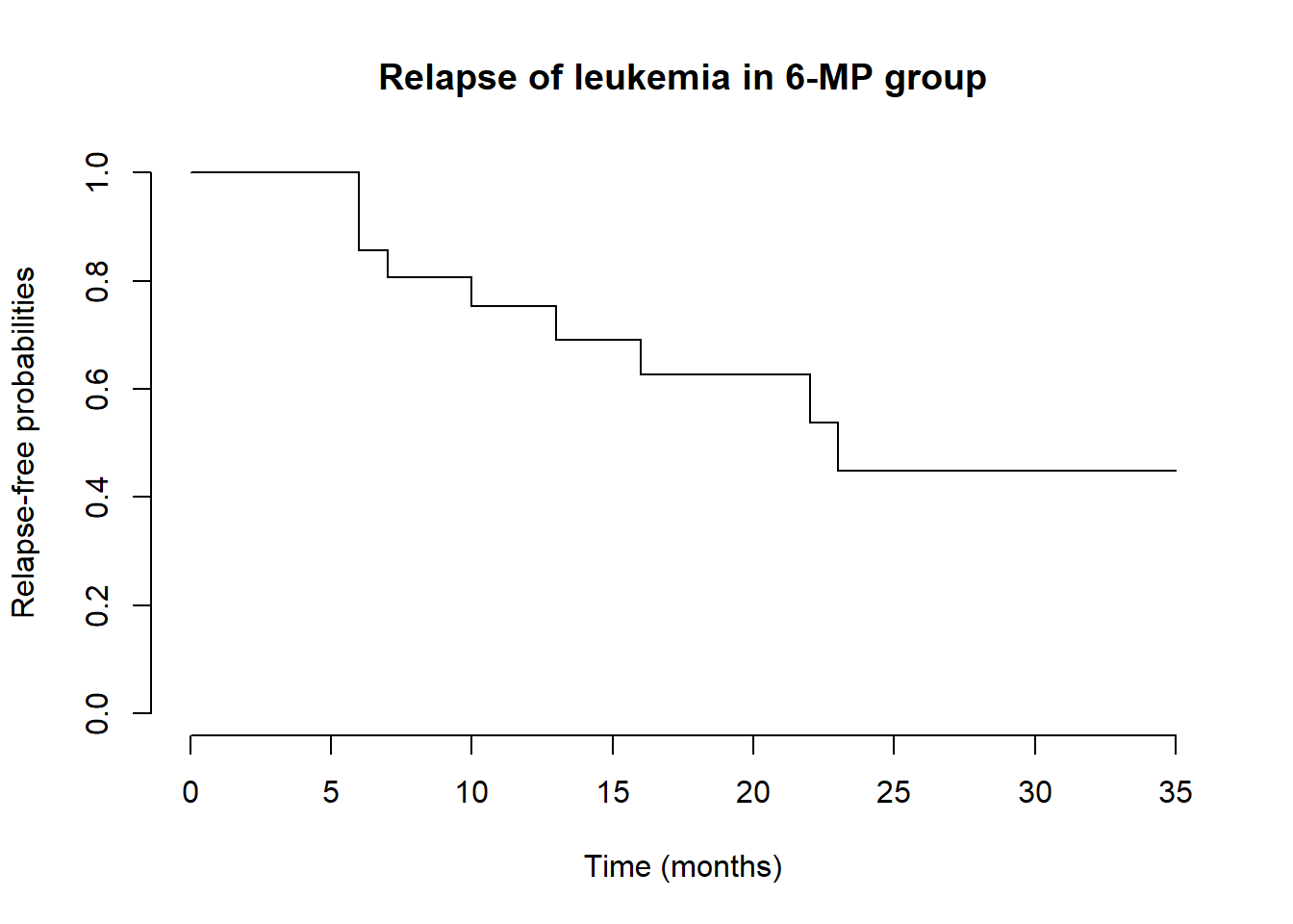
Parsing censored data

Instead of (time, status), sometimes the observed data are stored in a single column with censored observations indicated with a “+” or “>” sign.

For example, Table 1.1 of Klein and Moeschberger (2003) lists the times (in months) to relapse of leukemia in the treatment group (6-MP):

MP <- c(10, 7, "32+", 23, 22, 6, 16, "34+", "32+", "25+", "11+", "20+", 
        "19+", 6, "17+", "35+", 6, 13, "9+", "6+", "10+")

To convert the character strings to (time, status), use parse_number() to parse out the number and str_detect() to detect whether the string contains “+”:

# Example data: relapse times with "+" indicating censoring
MP <- c(10, 7, "32+", 23, 22, 6, 16, "34+", "32+", "25+", 
        "11+", "20+", "19+", 6, "17+", "35+", 6, 13, "9+", 
        "6+", "10+")

# Convert to (time, status) format
df <- tibble(
  MP = MP,
  time = parse_number(MP),               # Extract numeric part
  status = 1 - str_detect(MP, "\\+")    # Censored if "+" detected
)

# Display the parsed data
df

# A tibble: 21 × 3
#    MP     time status
#    <chr> <dbl>  <dbl>
#  1 10       10      1
#  2 7         7      1
#  3 32+      32      0
#  4 23       23      1
#  5 22       22      1
#  6 6         6      1
#  7 16       16      1
#  8 34+      34      0
#  9 32+      32      0
# 10 25+      25      0
# ℹ 11 more rows
# ℹ Use `print(n = ...)` to see more rows

Now feed this dataset into survfit() to estimate survival probabilities:

# Kaplan-Meier fit
km <- survfit(Surv(time, status) ~ 1, data = df)

# Plot the survival curve
plot(
  km,
  main = "Relapse of Leukemia in 6-MP Group",
  xlab = "Time (months)",
  ylab = "Relapse-free probabilities",
  conf.int = FALSE,
  frame = FALSE
)

Facet plotting Fig. 1.2

Here, we use survival data from the German Breast Cancer Study (GBC). Adjust the file path as needed.

# Read in the GBC mortality data
data <- read.table("Data//German Breast Cancer Study//gbc_mort.txt")

# Display the first few rows
head(data)
#   id      time status hormone age meno size grade nodes prog estrg
# 1  1 74.819672      0       1  38    1   18     3     5  141   105
# 2  2 65.770492      0       1  52    1   20     1     1   78    14
# 3  3 47.737705      1       1  47    1   30     2     1  422    89
# 4  4  4.852459      0       1  40    1   24     1     3   25    11
# 5  5 61.081967      0       2  64    2   19     2     1   19     9
# 6  6 63.377049      0       2  49    2   56     1     3  356    64

Then compute the different estimates within each level of hormone. Do this by using group_by(hormone) and performing the calculations within reframe(). But first we use survfit() to get the Kaplan–Meier estimates:

# Kaplan-Meier estimates
obj <- summary(survfit(Surv(time, status) ~ hormone, data = data))

# Extract survival probabilities into a tibble
km <- tibble(
  t = obj$time,
  surv = obj$surv,
  hormone = parse_number(as.character(obj$strata)), # Hormone group
  type = "Kaplan-Meier"
) |> 
  add_row(
    # Add starting points at (0, 1) for each group
    t = c(0, 0),
    surv = c(1, 1),
    hormone = 1:2,
    type = "Kaplan-Meier"
  )

Then the event-imputation and complete-case estimates (with ecdf() for empirical distribution function):

# Event-imputation estimates
imp <- data |> 
  group_by(hormone) |> 
  reframe(
    t = time,
    surv = 1 - ecdf(time)(time)  # Empirical survival function
  ) |> 
  arrange(t) |> 
  mutate(type = "Event-imputation")

# Complete-case estimates
cc <- data |> 
  filter(status == 1) |> 
  group_by(hormone) |> 
  reframe(
    t = time,
    surv = 1 - ecdf(time)(time)
  ) |> 
  arrange(t) |> 
  mutate(type = "Complete-case")

Now plot the figure:

# Combine estimates
estimates <- bind_rows(km, imp, cc)

# Define panel labels
hormone_labeller <- c("1" = "No Hormone", "2" = "Hormone")

# Plot
estimates |> 
  mutate(type = factor(type, levels = c("Kaplan-Meier", "Event-imputation", "Complete-case"))) |> 
  ggplot(aes(x = t, y = surv, linetype = type)) +
  geom_step() +
  facet_wrap(~ hormone, labeller = labeller(hormone = hormone_labeller)) +
  theme_bw() +
  scale_x_continuous(name = "Time (months)", breaks = seq(0, 72, 12), limits = c(0, 72)) +
  scale_y_continuous(name = "Survival rate", limits = c(0, 1)) +
  scale_linetype_manual(name = "Method", values = 1:3) +
  theme(legend.position = "bottom")

Prettier than Fig. 1.2?

Table 1

Let’s recreate Table 1.12, that is, “Table 1” for the German Breast Cancer study. Because the summary statistics are grouped by hormone status and overall, we add a replica to the original data where hormone is set to “Overall”, thereby creating three levels: “No hormone”, “Hormone”, “Overall”. Then we can use summarize() to calculate the summary statistics within each level of hormone after group_by(hormone).

To do so, we will define three summary functions:

One calculating median (IQR) for a quantitative variable;
One calculating N (%) for each level of a categorical variable;
One calculating event rate based on time and status.

To start, read in and clean the GBC mortality data for the subject-level statistics and death rate:

library(knitr) # for printing formatted table

## for subject-level summary and mortality
## read in the GBC mortality data
data <- read.table("Data//German Breast Cancer Study//gbc_mort.txt")

# Clean and expand data with "Overall" group
df <- data |> 
  mutate(hormone = if_else(hormone == 1, "No Hormone", "Hormone")) |> 
  add_row(data |> mutate(hormone = "Overall")) |> 
  mutate(
    hormone = factor(hormone, levels = c("No Hormone", "Hormone", "Overall")),
    meno = if_else(meno == 1, "No", "Yes")
  )

Now, write a function to compute median (IQR) and use it on the quantitative variables. In the process, we use pivot_longer() and pivot_wider() to put the hormone levels on the columns rather than rows. (For details on these data transposition tools, see https://r4ds.hadley.nz/data-tidy).

## Function to compute median (IQR) for x
## rounded to the rth decimal place
med_iqr <- function(x, r = 1){
  qt <- quantile(x, na.rm = TRUE)
  
  str_c(round(qt[3], r), " (", 
        round(qt[2], r), ", ",
        round(qt[4], r), ")")
}

# create summary table for quantitative variables
# age, size, nodes, prog, estrg
tab_quant <- df |> 
  group_by(hormone) |> 
  summarize(
    across(c(age, size, nodes, prog, estrg), med_iqr)
  ) |> 
  pivot_longer( # long format: value = median (IQR); name = variable names
    !hormone,
    values_to = "value",
    names_to = "name"
  ) |> 
  pivot_wider( # wide format: name = variable names; hormone levels as columns
    values_from = value,
    names_from = hormone
  ) |> 
  mutate(
    name = case_when( # format the variable names
      name == "age" ~ "Age (years)",
      name == "size" ~ "Tumor size (mm)",
      name == "nodes" ~ "# Nodes",
      name == "prog" ~ "Progesterone (fmol/mg)",
      name == "estrg" ~ "Estrogen (fmol/mg)"
    )
  )

See what the result looks like:

tab_quant
# # A tibble: 5 × 4
#   name                   `No Hormone` Hormone       Overall        
#   <chr>                  <chr>        <chr>         <chr>          
# 1 Age (years)            50 (45, 59)  58 (50, 63)   53 (46, 61)    
# 2 Tumor size (mm)        25 (20, 35)  25 (20, 35)   25 (20, 35)    
# 3 # Nodes                3 (1, 7)     3 (1, 7)      3 (1, 7)       
# 4 Progesterone (fmol/mg) 32 (7, 130)  35 (7.2, 133) 32.5 (7, 131.8)
# 5 Estrogen (fmol/mg)     32 (8, 92.2) 46 (9, 182.5) 36 (8, 114)

Next we deal with categorical variables. Because the results span multiple rows due to multiple levels, it is easier to write a data frame function, one that takes the tibble data frame as an argument. For details, see https://r4ds.hadley.nz/functions#data-frame-functions.

## a function that computes N (%) for each level of var
## by group in data frame df (percent rounded to rth point)
freq_pct<- function(df, group, var, r = 1){
  # compute the N for each level of var by group
  var_counts <- df |> 
    group_by({{ group }}, {{ var }}) |> 
    summarize(
      n = n(),
      .groups = "drop"
    ) 
  # compute N (%)
  var_counts |> 
    left_join( # compute the total number (demoninator) in each group
               # and joint it back to the numerator
      var_counts |> group_by({{ group }}) |> summarize(N = sum(n)),
      by = join_by({{ group }})
    ) |> 
    mutate( # N (%)
      value = str_c(n, " (", round(100 * n / N, r), "%)")
    ) |> 
    select(- c(n, N)) |> 
    pivot_wider( # put group levels on columns
      names_from = {{ group }},
      values_from = value
    ) |> 
    rename(
      name = {{ var }} # name = variable names 
    )
}

Apply this function to meno and grade (by hormone of course):

## menopausal status
meno <- df |>
  freq_pct(hormone, meno) |> 
  mutate(
    name = str_c("Menopause - ", name)
  )

## tumor grade
grade <- df |> 
  freq_pct(hormone, grade) |> 
  mutate(
    name = str_c("Tumor grade - ", name)
  )

Combine with the quantitative variables:

tabone <- tab_quant |> 
  add_row(meno) |> 
  add_row(grade)

tabone
# # A tibble: 10 × 4
#    name                   `No Hormone` Hormone       Overall        
#    <chr>                  <chr>        <chr>         <chr>          
#  1 Age (years)            50 (45, 59)  58 (50, 63)   53 (46, 61)    
#  2 Tumor size (mm)        25 (20, 35)  25 (20, 35)   25 (20, 35)    
#  3 # Nodes                3 (1, 7)     3 (1, 7)      3 (1, 7)       
#  4 Progesterone (fmol/mg) 32 (7, 130)  35 (7.2, 133) 32.5 (7, 131.8)
#  5 Estrogen (fmol/mg)     32 (8, 92.2) 46 (9, 182.5) 36 (8, 114)    
#  6 Menopause - No         231 (52.5%)  59 (24%)      290 (42.3%)    
#  7 Menopause - Yes        209 (47.5%)  187 (76%)     396 (57.7%)    
#  8 Tumor grade - 1        48 (10.9%)   33 (13.4%)    81 (11.8%)     
#  9 Tumor grade - 2        281 (63.9%)  163 (66.3%)   444 (64.7%)    
# 10 Tumor grade - 3        111 (25.2%)  50 (20.3%)    161 (23.5%)

As the last step, create an event rate function and apply it to df to calculate the death rate:

# event rate function
# status = 1 for event
event_rate <- function(time, status){
  sum(status)/sum(time) 
  # we don't use sum(x, na.rm = TRUE) because
  # missing data should alarm us
}

# calculate death rates
death_rates <- df |> 
  group_by(hormone) |> 
  summarize(
    death_rate = as.character(round(event_rate(time, status) * 12, 3)) # per year
  ) |> 
  pivot_wider(
    names_from = hormone,
    values_from = death_rate
  ) |> 
  mutate(
    name = "Death rate (per person-year)",
    .before = 1
  )

death_rates
# # A tibble: 1 × 4
#   name                         `No Hormone` Hormone Overall
#   <chr>                        <chr>        <chr>   <chr>  
# 1 Death rate (per person-year) 0.075        0.059   0.069

Finally, read in and clean up the complete data (relapse and death) to calculate the composite endpoint (CE; time to first) event rate.

# Read in the complete data
gbc <- read.table("Data//German Breast Cancer Study//gbc.txt")

## get the first event (minimum time)
## for each patient id
gbc_ce <- gbc |> 
  group_by(id) |> 
  slice_min(time) |> # take min time
  slice_max(status) |> # if death (2) is tied with relapse (1), take death
  ungroup()

## same manipulations
df_ce <- gbc_ce |> 
  mutate(
    hormone = if_else(hormone == 1, "No Hormone", "Hormone")
  ) |> 
  add_row(gbc_ce |> mutate(hormone = "Overall")) |> 
  mutate(
    hormone = fct(hormone, levels = c("No Hormone", "Hormone", "Overall")),
  )

Apply the same event rate function to calculate the CE rate.

ce_rates <- df_ce |> 
  group_by(hormone) |> 
  summarize(
    ce_rate = as.character(round(event_rate(time, status > 0) * 12, 3)) # per year
  ) |> 
  pivot_wider(
    names_from = hormone,
    values_from = ce_rate
  ) |> 
  mutate(
    name = "CE rate (per person-year)",
    .before = 1
  )

Add the event rates to the table and print it out:

## add event rates
tabone <- tabone |> 
  add_row(
    death_rates
  ) |> 
  add_row(
    ce_rates
  ) 

## add N to group names  
colnames(tabone) <- c(" ", str_c(colnames(tabone)[2:4], " (N=", table(df$hormone),")"))
## print out the table
kable(tabone)

Table 1: Patient characteristics in the German Breast Cancer study.

	No Hormone (N=440)	Hormone (N=246)	Overall (N=686)
Age (years)	50 (45, 59)	58 (50, 63)	53 (46, 61)
Tumor size (mm)	25 (20, 35)	25 (20, 35)	25 (20, 35)
# Nodes	3 (1, 7)	3 (1, 7)	3 (1, 7)
Progesterone (fmol/mg)	32 (7, 130)	35 (7.2, 133)	32.5 (7, 131.8)
Estrogen (fmol/mg)	32 (8, 92.2)	46 (9, 182.5)	36 (8, 114)
Menopause - No	231 (52.5%)	59 (24%)	290 (42.3%)
Menopause - Yes	209 (47.5%)	187 (76%)	396 (57.7%)
Tumor grade - 1	48 (10.9%)	33 (13.4%)	81 (11.8%)
Tumor grade - 2	281 (63.9%)	163 (66.3%)	444 (64.7%)
Tumor grade - 3	111 (25.2%)	50 (20.3%)	161 (23.5%)
Death rate (per person-year)	0.075	0.059	0.069
CE rate (per person-year)	0.161	0.113	0.142

Using `gtsummary`

There is a simpler way to create Table 1.12 using the gtsummary package.

library(gtsummary) 
library(labelled) # For labelling variables

# Re-read data to keep it distinct (optional)
gbc_mort <- read.table("Data//German Breast Cancer Study//gbc_mort.txt")

df_gts <- gbc_mort |> 
  mutate(
    hormone = if_else(hormone == 1, "No Hormone", "Hormone"),
    hormone = factor(hormone, levels = c("No Hormone", "Hormone")),
    meno = if_else(meno == 1, "No", "Yes") |> factor(levels = c("No", "Yes"))
  )

# Labeling variables
var_label(df_gts) <- list(
  time = "Time to event (months)",
  status = "Event status",
  hormone = "Hormone therapy",
  age = "Age (years)",
  meno = "Menopausal status",
  size = "Tumor size (mm)",
  grade = "Tumor grade",
  nodes = "Number of nodes",
  prog = "Progesterone (fmol/mg)",
  estrg = "Estrogen (fmol/mg)"
)

tbl1 <- df_gts |>
  tbl_summary(
    by = hormone,
    include = ! c(id, time, status),
    missing = "no"
  ) |>
  add_overall(last = TRUE) |> # At the end
  italicize_levels()

tbl1

Characteristic	No Hormone, N = 440¹	Hormone, N = 246¹	Overall, N = 686¹
Age (years)	50 (45, 59)	58 (50, 63)	53 (46, 61)
Menopausal status	209 (48%)	187 (76%)	396 (58%)
Tumor size (mm)	25 (20, 35)	25 (20, 35)	25 (20, 35)
Tumor grade
1	48 (11%)	33 (13%)	81 (12%)
2	281 (64%)	163 (66%)	444 (65%)
3	111 (25%)	50 (20%)	161 (23%)
Number of nodes	3 (1, 7)	3 (1, 7)	3 (1, 7)
Progesterone (fmol/mg)	32 (7, 130)	35 (7, 133)	33 (7, 132)
Estrogen (fmol/mg)	32 (8, 92)	46 (9, 183)	36 (8, 114)
¹ Median (IQR); n (%)

However, we still need to “manually” calculate the event rates.

References

Klein, John P., and Melvin L. Moeschberger. 2003. Survival Analysis: Techniques for Censored and Truncated Data. Springer New York. https://doi.org/10.1007/b97377.