Applied Survival Analysis
Chapter 1 - Introduction
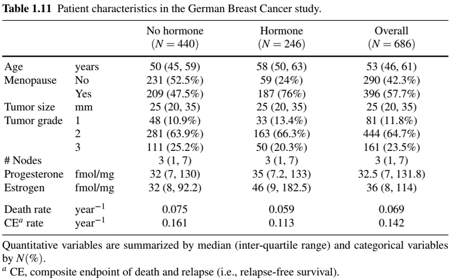
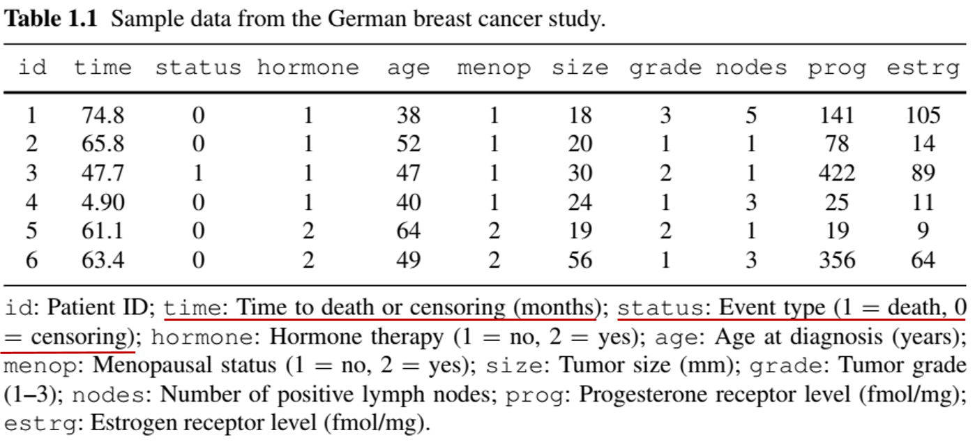
Example: Univariate event (II)
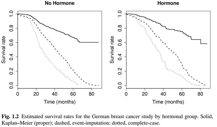
- German Breast Cancer (GBC) Study
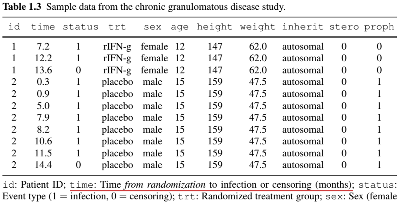
Example: Recurrent events (II)
- Chronic Granulomatous Disease (CGD) Study
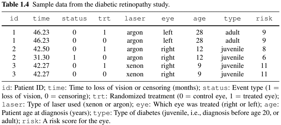
Example: Multivariate/Clustered Events (II)
- Diabetic Retinopathy Study
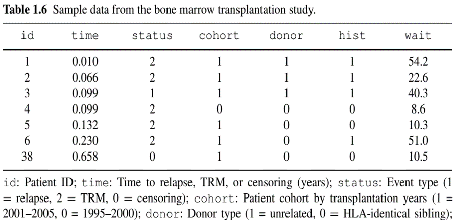
Example: Competing Risks (III)
- Bone Marrow Transplant Study
- Why only one record per patient?
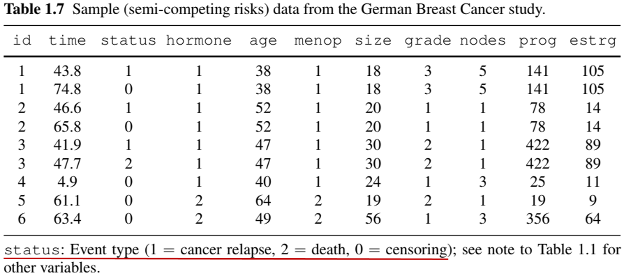
Example: More Complex Outcomes (Semi-competing risks)
- German Breast Cancer (GBC) Study
- Nonfatal event + terminal event (death)
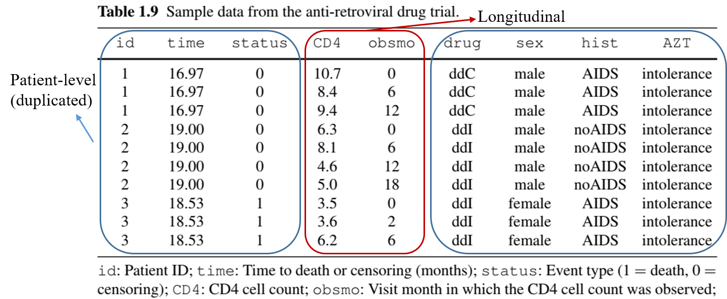
Example: More Complex Outcomes (with Longitudinal data)
- Anti-Retroviral Drug Trial
- Repeated measures of CD4 cell count + death
Example: More Complex Outcomes (Multistate process)
- Breast Cancer Life History Study
- Remission \(\to\) relapse \(\to\) metastasis \(\to\) death (can skip states)

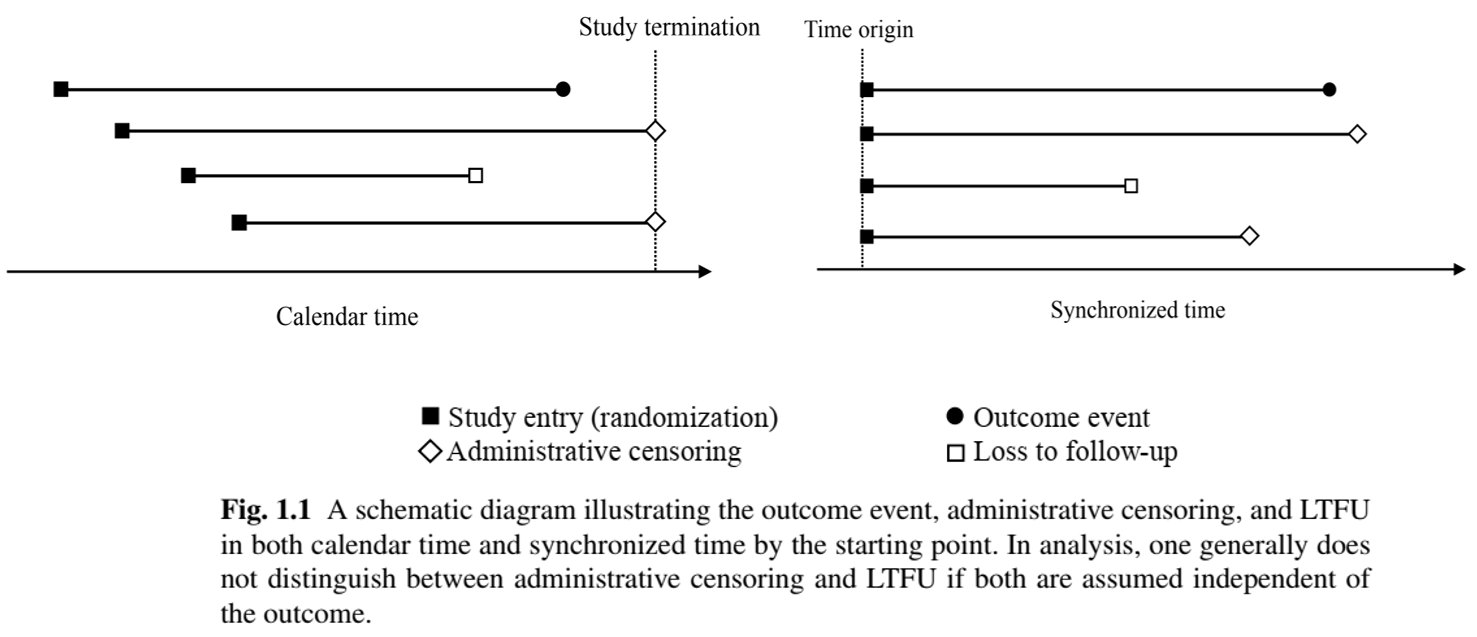
Censoring Mechanisms: Illustration
- Calendar time vs time synchronized by starting point
Statistical Implications: Example
- German Breast Cancer (GBC) Study
How to Calculate Event Rate (I)
- Length of follow-up is event-specific
- If an event is “non-recurrent”, its occurrence means patient is no longer at risk for it
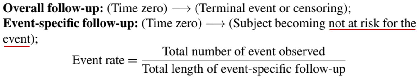
Note
Denominator is called person-year (or person-time) of follow-up.
How to Calculate Event Rate (II)
- Semi-competing risks

How to Calculate Event Rate (III)
- Recurrent events
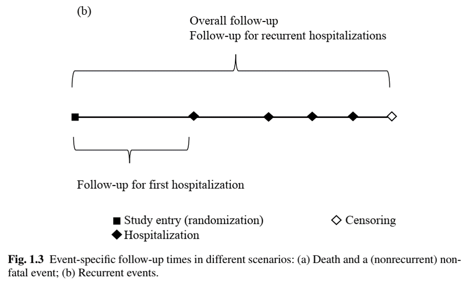
Table One: Example