Applied Survival Analysis

Chapter 7 - Left Truncation and Interval Censoring

Lu Mao

lmao@biostat.wisc.edu

Department of Biostatistics & Medical Informatics

University of Wisconsin-Madison

Outline

1. Left truncation mechanisms

2. Standard and general methods for left truncation

3. Non- and Semi-parametric methods for Interval censoring

4. Bangkok Metropolitan Administration HIV Study

\[\newcommand{\d}{{\rm d}}\] \[\newcommand{\T}{{\rm T}}\] \[\newcommand{\dd}{{\rm d}}\] \[\newcommand{\pr}{{\rm pr}}\] \[\newcommand{\var}{{\rm var}}\] \[\newcommand{\se}{{\rm se}}\] \[\newcommand{\indep}{\perp \!\!\! \perp}\] \[\newcommand{\Pn}{n^{-1}\sum_{i=1}^n}\]

Left Truncation: Mechanisms

Truncation - Biased Sampling

• Left truncation
  • Only subjects who fail in \([T_L, \infty)\) can be observed
    • \(T_L\): left truncation time
    • Those who fail in \([0, T_L)\) are excluded (truncated)
    • Biased sampling \((T\geq T_L)\)

• Mechanism: delayed entry
  • Subject entering study after starting point

Examples of Delayed Entry

• Starting point: before enrollment
  • Birth: age at death
    • Dead before enrollment excluded
  • Diagnosis of cancer: time from diagnosis to death
    • Dead before enrollment excluded
  • Blood transfusion: time from tranfusion to AIDS
    • Positive before enrollment excluded

Truncation vs Censoring

• Difference
  • Truncation : Biased sampling
  • Censoring: Partial missing data

• Left truncation \(+\) right censoring

Left Truncation: Methods

Data and Assumption

• Target of inference: still \(T\)

• Observed data \[ (T_{Li}, X_i, \delta_i) \,\,\, (i=1,\ldots, n) \]

  • \(T_{Li}\): left truncation (delayed entry) time for subject \(i\)

• Independent truncation \[T_L\indep T\]

  • In case with covariates \((T_L\indep T)\mid Z\)

Standard Methods

• Methods by at-risk conditioning
  • Kaplan–Meier estimate
  • Log-rank test
  • Cox model

• Easy fix: adjust at-risk status
  • Subject not at risk before entry
  • At risk (on study): \([T_{Li},\; X_i]\)

Standard Methods: Nonparametric (I)

• Nelsen-Aalen estimator: \(\dd\hat\Lambda(t_j)=d_j/n_j\)
  • Without late entry: \(n_j=\sum_{i=1}^nI(X_i\geq t_j)\)
  • With late entry: \(n_j=\sum_{i=1}^nI(T_{Li}\leq t_j\leq X_i)\)

• Kaplan-Meier estimator \[ \hat S(t)=\prod_{j: t_j\leq t}\left(1 - d_j/n_j\right) \]

Standard Methods: Nonparametric (II)

• Identifiability
  • Suppose earliest entry time \(t_0=\min(T_{Li})>0\)
  • No data in \([0, t_0]\)

• Conditional survival function \[\begin{align} \hat S(t)&\to \pr(T>t_1\mid T>t_0)\pr(T>t_2\mid T>t_1)\cdots\pr(T>t\mid T>t_j)\\ & = \pr(T>t \mid T>t_0) \end{align}\]
  • Not the marginal \(\pr(T>t)\)
  • Solution: choose a late \(t_0^*> t_0\) (s.t. \(n_j\gg 1\) for all \(t_j\geq t_0^*\)) and consider \[\begin{equation} \hat\pr(T>t\mid T \geq t_0^*)=\prod_{j:t_0^*\leq t_j\leq t}(1-d_j/n_j), \end{equation}\]

Standard Methods - Cox Model (I)

• Partial likelihood construction
  • Without late entry: \(\mathcal R_j=\{i: X_i\geq t_j\}\)
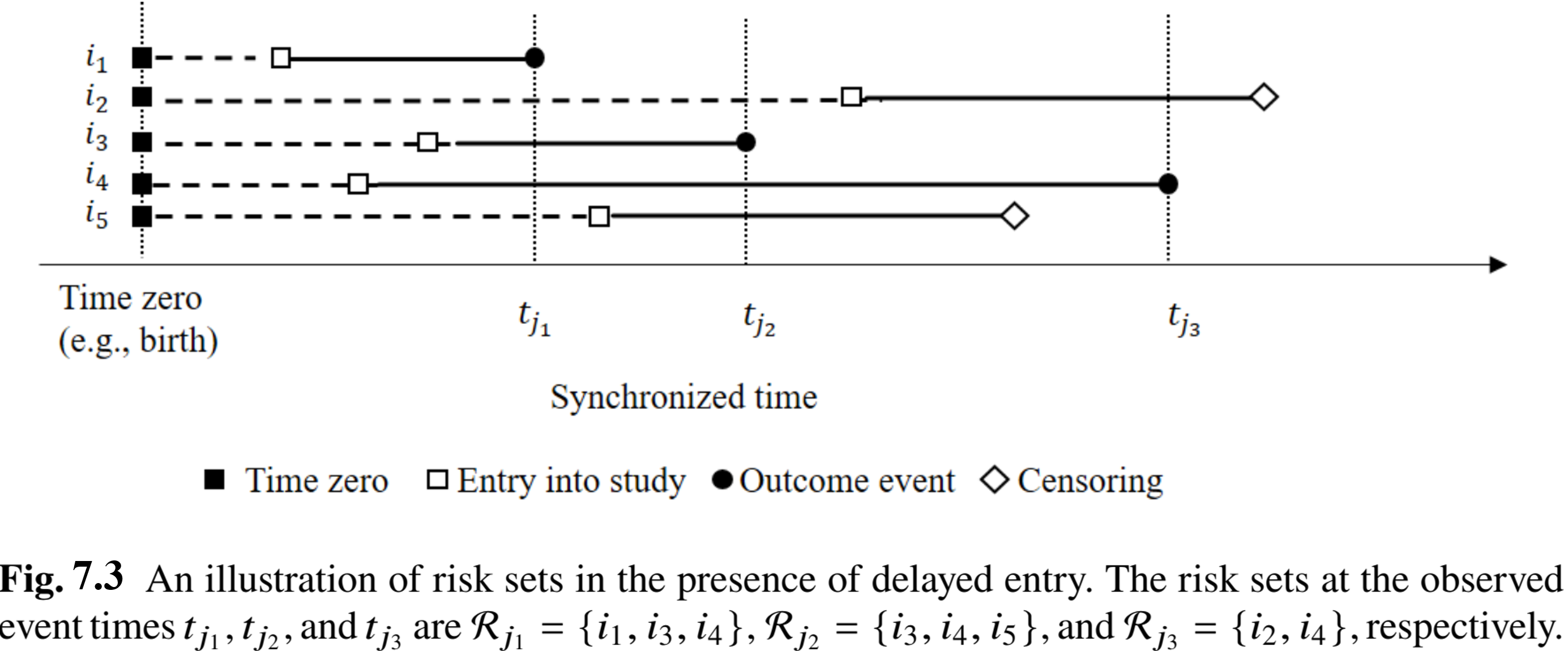
  • With late entry: \(\mathcal R_j=\{i: T_{Li}\leq t_j\leq X_i\}\)

Standard Methods - Cox Model (II)

• Risk sets: example

Standard Methods - Cox Model (III)

• Partial-likelihood score
  • Adjust the at-risk process \[ U_n(\beta)=\Pn\int_0^\infty\left\{Z_i-\frac{\sum_{j=1}^n I(T_{Lj}\leq t\leq X_j)Z_j\exp(\beta^\T Z_j)} {\sum_{j=1}^n I(T_{Lj}\leq t\leq X_j)\exp(\beta^\T Z_j)}\right\}\dd N_i(t) \]

• Other extensions
  • Log-rank test: \(U_n(0)\) with binary \(Z\)
  • Martingale residuals: \[ \dd M_i(t)=\dd N_i(t)-I(T_{Li}\leq t\leq X_i)\exp(\beta^\T Z_i)\dd\Lambda_0(t) \]
  • Time-varying covariates

Standard Methods - Cox Model (IV)

• Prediction of survival rate

  • If all subjects enter late, choose late cutoff \(t_0^*\)

  • Conditional survival function \[\begin{equation} \hat\pr(T > t\mid T\geq t_0^*, Z) = \exp\left[-\left\{\hat\Lambda_0(t)- \hat\Lambda_0(t_0^*)\right\}\exp(\hat\beta^\T Z)\right] \end{equation}\]

Exercise

Show that \[\pr(T > t\mid T\geq t_0^*, Z) = \exp\left[-\left\{\Lambda_0(t)- \Lambda_0(t_0^*)\right\}\exp(\beta^\T Z)\right] \] for any \(t>t_0^*\) under the Cox model.

General Approach - Likelihood

• Non-hazard-based methods
  • Proportional odds model
  • Accelerated failure time model

• Re-construct likelihood
  • A model parametrized by \(\theta\) \[\begin{equation}\label{eq:trunc:lik} L_n(\theta)=\prod_{i=1}^n S(T_{Li};\theta)^{-1}\lambda(X_i;\theta)^{\delta_i}S(X_{i};\theta) \end{equation}\]
    • Every subject sampled is conditioned upon \(T_i\geq T_{Li}\), hence inverse weight \(S(T_{Li};\theta)\)
  • Log-likelihood: \(l_n(\theta)=\sum_{i=1}^n\left[\delta_i\log\lambda(X_i;\theta)-\left\{\Lambda(X_i;\theta)-\Lambda(T_{Li};\theta)\right\}\right]\)

Maximum Likelihood: PO Model

• Example: Proportional odds model
  • Model specification with \(\theta = (\beta, h_0)\) \[\begin{equation}\label{eq:non_haz:po} \log\left\{\frac{1-S(t\mid Z)}{S(t\mid Z)}\right\}=h_0(t)+\beta^\T Z, \end{equation}\]
  • Model-based hazard functions \[\begin{align} \lambda(t\mid Z;\beta, h_0)&=\frac{\exp\{h_0(t)+\beta^\T Z\}h_0'(t)}{1+\exp\{h_0(t)+\beta^\T Z\}}\\ \Lambda(t\mid Z;\beta, h_0)&=\log\left[1+\exp\{h_0(t)+\beta^\T Z\}\right] \end{align}\]
  • Nonparametric maximum likelihood (NPMLE)
    • Discretize \(h_0(\cdot)\) at observed event times \(t_1<\cdots<t_m\)
    • \(h_0'(t_j)=h_{0j}\); \(h_0(t)=\sum_{j:t_j\leq t}h_{0j}\)

Software: survival::Surv()

• Basic syntax for handling left truncation

## Fit Kaplan-Meier curve to left-truncated data
survfit(Surv(entry, end, status) ~ 1)
## Fit Cox model to left-truncated data
coxph(Surv(entry, end, status) ~ covariates)

• Input

  • entry: \(T_{L}\); end: \(X\); status: \(\delta\)

• Output: survfit or coxph object

• log-rank test: score test under coxph()

Example: Channing House Study (I)

• Study information
  • Population: 462 elderly residents of Channing House, a retirement center
  • Endpoint: Age at death (starting point: birth)
  • Aim: Compare mortality between males (gender=1) and females (gender=2)
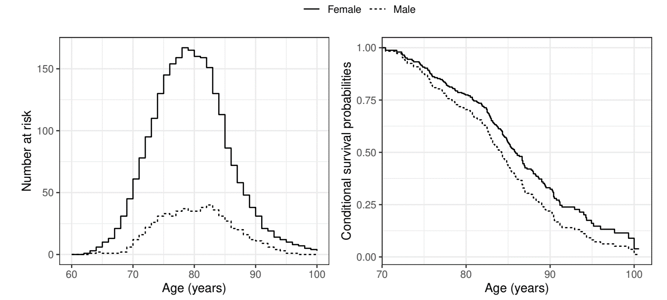
  • Truncation: Age of admission into the center (Entry.Age)
    • Subject must survive long enough to enter cohort (link to follow-up plot)

head(channing)
#   Entry.Age  End.Age status gender
# 1  86.83333 97.66667      1      2
# 2  76.75000 86.66667      1      2
# 3  73.75000 83.58333      1      2
# ...

Example: Channing House Study (II)

• Cox model
  • females at 72.9% risk as males for mortality (\(p\)-value 0.07)

obj <- coxph(Surv(Entry.Age, End.Age, status) ~ factor(gender), 
             data = channing)
summary(obj)
#                    coef exp(coef) se(coef)      z Pr(>|z|)  
# factor(gender)2 -0.3163    0.7289   0.1731 -1.827   0.0677 .
# ---
# 
#                 exp(coef) exp(-coef) lower .95 upper .95
# factor(gender)2    0.7289      1.372    0.5191     1.023
# 
# Concordance= 0.528  (se = 0.018)
# Likelihood ratio test= 3.17  on 1 df,   p=0.07
# Wald test            = 3.34  on 1 df,   p=0.07
# Score (logrank) test = 3.36  on 1 df,   p=0.07

Example: Channing House Study (III)

• Checking proportionality

# Schoenfeld residuals
obj_zph <- cox.zph(obj)
# test result
obj_zph
# plot the rescaled residuals
plot(obj_zph, ylab = "Gender", xlab = "Age (years)", lwd = 2)

Example: Channing House Study (IV)

• Prediction (at age 70)

Interval Censoring

Observation Setting

• Interval censoring
  • Periodic check-ups for an asymptomatic event
  • Event is only known to have occurred in between two consecutive check-ups

• Examples
  • Tumor (occult) formation
  • HIV seroconversion (viral antibodies become detectable in serum)

• Challenge
  • No exact failure time is observed

Data and Assumption

• Target of inference: still \(T\)

• Check-up times: \(U=(U_1<U_2<\cdots<U_K)\)
  • \(K\equiv 1\): case-1 (current status data)
  • \(K\equiv 2\): case-2
  • \(\vdots\)
  • \(K\) random (subject-specific): mixed-case
• Independent check-up \[ U\indep T \]
  • With covariates: \((U\indep T)\mid Z\)

Observed Data

• Censoring interval
  • \((L, R]\): the check-up interval containing the event
  • Other check-up times may be available but not relevant
  • Example: current status data
    • “Positive” at \(U_1\): \((L, R]=(0, U_1]\)
    • “Negative” at \(U_1\): \((L, R]=(U_1, \infty)\)

• Observed sample \[ (L_i, R_i)\,\,\,(i=1,\ldots, n) \]

Likelihood-Based Inference

• Likelihood function \[\begin{equation}\label{eq:trunc:nonp} L_n(\theta)=\prod_{i=1}^n\{S(L_i;\theta)-S(R_i;\theta)\} \end{equation}\]
  • Log-likelihood \[\begin{equation}\label{eq:trunc:ic_log_lik} l_n(\theta)=\sum_{i=1}^n\log\{S(L_i;\theta)-S(R_i;\theta)\} \end{equation}\]

• Parametric Models
  • Standard MLE \(\hat\theta=\arg\max_\theta l_n(\theta)\)

One-Sample Estimation

• Nonparametric maximum likelihood
  • \(F(t)=1-S(t)\): treat as a step function
  • Log-likelihood \[ l_n(F)=\sum_{i=1}^n\log\{F(R_i)-F(L_i)\} \]
  • \(F(\cdot)\): step function jumping at unique (finite) values of the \(R_i\): \[ t_1<t_2<\cdots<t_m \]
  • \(l_n(F)\) becomes a function of \[ 0\leq F(t_1)\leq F(t_2)\leq\cdots \leq F(t_m)\leq 1 \]

One-Sample: Constrained Maximization

• Monotonicity-constrained maximization \[\begin{equation}\label{eq:trunc:iso} \hat F=\arg\max_{F\in\mathcal A}l_n(F). \end{equation}\]
  • \(\mathcal A=\{F: 0\leq F(t_1)\leq F(t_2)\leq\cdots \leq F(t_m)\leq 1\}\): a convex set
  • Solvable by linear programming
  • Iterative convex minorant (ICM): a monotonicity-contrained version of Newton-Raphson
  • \(\hat F(t) - F(t)= O_P(n^{-1/3})\), not asymptotically normal

Semiparametric Models

• General approach \(\theta=(\beta, \eta)\)
  • \(\beta\): regression parameter
  • \(\eta(\cdot)\): nonparametric (monotone) baseline function (cumulative hazards/odds)
  • \((\hat\beta, \hat\eta)=\arg\max_{\beta,\eta}l_n(\beta, \eta)\): maximize iteratively between \(\beta\) and \(\eta(\cdot)\)

• Example: Cox proportional hazards (PH) model
  • Log-likelihood \[ l_n(\beta,\Lambda_0)=\sum_{i=1}^n\log\left[\exp\{-\exp(\beta^\T Z_i)\Lambda_0(L_i)\}-\exp\{-\exp(\beta^\T Z_i)\Lambda_0(R_i)\}\right] \]

Example: Cox PH Model

• Iterative maximization
  • \(\beta\)-step (Newton-Raphson) \[ \beta^{(j+1)}=\arg\max_\beta l_n(\beta,\Lambda_0^{(j)}) \]
  • \(\Lambda_0\)-step (ICM) \[ \Lambda_0^{(j+1)}=\arg\max_\Lambda l_n(\beta^{(j+1)},\Lambda) \]

• Inference
  • \(\hat\Lambda_0(t)-\Lambda_0(t)=O_P(n^{-1/3})\): non-standard distribution
  • \(\hat\beta\) asymptotically normal, variance estimable by efficient information
    • \(\mathcal I(\beta)=-\partial^2 l_n\{\beta, \hat\Lambda_0(\beta)\}/\partial\beta^{\otimes 2}\) (negative quadrature of “profile likelihood”)

Software: IntCens::icsurvfit()

• Basic syntax for analysis of interval-censored data

devtools::install_github("lmaowisc/IntCens")
library(IntCens)
# Fit non-/semi-parametric models to interval-censored data
obj <- icsurvfit(L, R, Z = NULL, model = c("NP", "PH", "PO"))

• Input
  • L, R: \(L_i\) and \(R_i\)
  • Z: covariate matrix (optional)
  • model = c("NP", "PH", "PO"): nonparametric (one-sample) estimation, PH, PO regression models
• Output: obj$beta (\(\hat\beta\)), obj$var(\(\hat\var(\hat\beta)\)), …

Bangkok HIV/AIDS Study

Study Background

• Study information
  • Population: 1,124 injecting drug users (IDUs) followed from 1995 to 1998 at 4-month intervals for blood test for HIV sero-positivity
  • Endpoint: (interval-censored) time from enrollment to HIV seroconversion (link to follow-up plot)
  • Baseline risk factors
    • Age (years)
    • Sex (1: male; 0: female)
    • History of needle sharing (1: yes; 0: no)
    • History of being jailed/imprisoned (1: yes; 0: no)
    • History of drug injection in jail (1: yes; 0: no)

Cox PH Regression

• Load package and data

library(IntCens)
## BMA data
head(df)
#     L       R age sex needle jail inject
#   40.6    Inf  37   0      0    1      1
#   24.3    Inf  25   0      0    1      1
#    0      4.1  49   0      1    1      1
#    7.1   13.2  32   1      0    1      0
# ...

• Fit Cox model

# Fit a proportional hazards model
PH_fit <- icsurvfit(L = df$L, R = df$R, Z = df[, 3:7], model = "PH")

Cox PH Regression: Inference (I)

• Summary results

# Print out regression results
PH_fit 
#> Call:
#> icsurvfit(L = df$L, R = df$R, Z = df[, 3:7], model = "PH")
#> 
#> ICM algorithm converges in 102 iterations.
#> 
#> Maximum Likelihood Estimates for Regression parameters:
#> 
#>         Estimate    StdErr z.value  p.value   
#> age    -0.029914  0.011051 -2.7068 0.006793 **
#> sex     0.387923  0.268032  1.4473 0.147814   
#> needle  0.249568  0.144987  1.7213 0.085195 . 
#> jail    0.456849  0.143961  3.1734 0.001506 **
#> inject  0.221270  0.146767  1.5076 0.131652   
#> ---
#> Signif. codes:  0 ‘***’ 0.001 ‘**’ 0.01 ‘*’ 0.05 ‘.’ 0.1 ‘ ’ 1

Cox PH Regression: Inference (II)

• Regression results
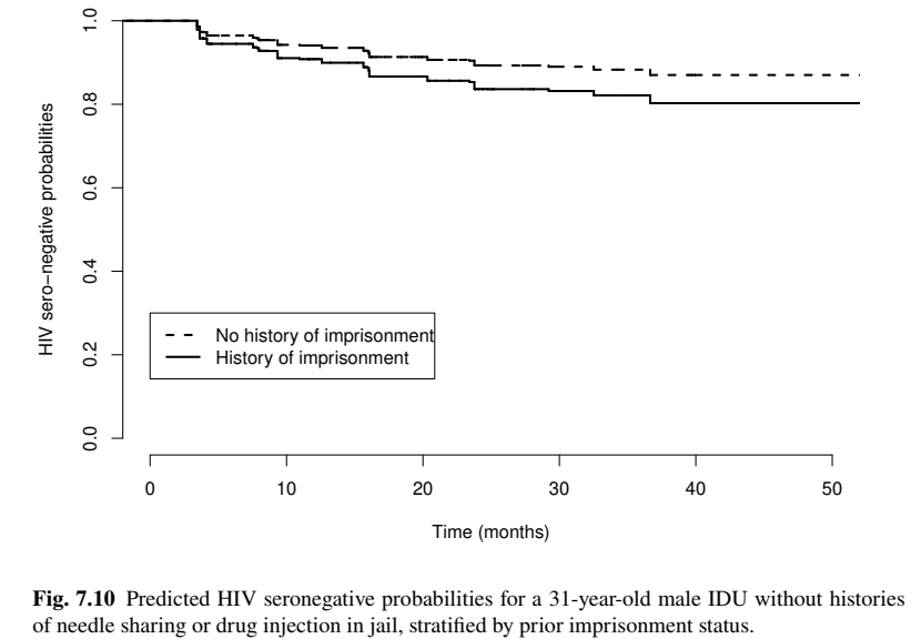
  • History of imprisonment increases risk of HIV seroconversion by \(1.58-1=58\%\) (\(p\)-value 0.002)

Cox PH Regression: Prediction

• Model-based prediction

Conclusion

Notes (I)

• Left-truncated and interval-censored (LTIC) data
  • Delayed entry with periodic check-ups
  • Pan and Chappell (1998a, 1998b, 2002), Gao and Chan (2018), etc.
• Interval-censored data
  • Review: Huang and Wellner (1997)
  • Time-varying covariates: Zeng et al. (2016)
  • Profile-likelihood: Murphy and van der Vaart (2000)
  • Text: Sun (2010)

Notes (II)

• Sun (2010)

Summary

• Left truncation
  • Caused by delayed entry
  • Kaplan-Meier, log-rank test, and Cox model \(\to\) modify risk set
  • survival::Surv(entry, end, status)
• Interval censoring
  • Periodic check-ups of non-fatal, asymptomatic event
  • Non- and semi-parametric models by NPMLE (ICM algorithm)
  • IntCens::icsurvfit()
    • Nonparametric estimation
    • Proportional hazards model
    • Proportional odds model

HW 4 (Due Mar 19)

• Choose one
  • Problem 5.1
  • Problem 5.2
• Problem 6.5
• Problem 7.14

# Install and load IntCens package
# devtools::install_github("lmaowisc/IntCens")
library(IntCens)