Chapter slides here. (To convert html to pdf, press E \(\to\) Print \(\to\) Destination: Save to pdf)
R code
Show the code
################################################################## This code generates the numerical results in chapter 1 ###################################################################library(survival) # For standard (univariate) survival analysislibrary(Wcompo) # For weighted total events (CompoML function)library(rmt) # For the hfaction data set (Heart Failure ACTION trial)library(tidyverse) # For data wrangling (dplyr, ggplot2, etc.)# load hfaction datadata(hfaction)head(hfaction) #> Shows the first rows of the hfaction data frame# convert status=1 for death, 2=hospitalization# (Swapping the original coding of event types in hfaction)hfaction <- hfaction |>mutate(status =case_when( status ==1~2, # status previously "1" becomes "2" now status ==2~1, # status previously "2" becomes "1" now status ==0~0# status "0" remains "0" (censoring) ) )head(hfaction)#> Check that the status values have been reassigned correctly# count unique patients in each armhfaction |>group_by(trt_ab) |>distinct(patid) |>count(trt_ab)#> Summarizes how many unique patients are in each treatment arm (trt_ab)# TFE: take the first event per patient id# This means each patient is represented by their earliest event (or censoring)hfaction_TFE <- hfaction |>arrange(patid, time) |>group_by(patid) |>slice_head() |>ungroup()# -------------------------------------------------------------------------# Mortality analysis# -------------------------------------------------------------------------## Get mortality datahfaction_D <- hfaction |>filter(status !=2) # remove hospitalization records (now coded as "2")## Cox model for death against trt_abobj_D <-coxph(Surv(time, status) ~ trt_ab, data = hfaction_D)summary(obj_D)#> n= 426, number of events= 93 #> coef exp(coef) se(coef) z Pr(>|z|) #> trt_ab -0.3973 0.6721 0.2129 -1.866 0.0621 .# Interpretation: a hazard ratio < 1 suggests lower hazard of death in the # training arm, though p-value is ~0.06.# -------------------------------------------------------------------------# TFE analysis# -------------------------------------------------------------------------## how many of first events are death (1) or hosp (2)hfaction_TFE |>count(status)#> Tells how many first events were coded as status=1 or status=2# Cox model for TFE against trt_ab# Here "status > 0" means any event (death or hospitalization) vs. censoringobj_TFE <-coxph(Surv(time, status >0) ~ trt_ab, data = hfaction_TFE)summary(obj_TFE)#> Similar interpretation as above, now for time to first event # (either death or hospitalization).# -------------------------------------------------------------------------# Mortality vs TFE# -------------------------------------------------------------------------library(ggsurvfit) # For Kaplan-Meier plots using ggplot2library(patchwork) # For combining plots side by sidepD <-survfit2(Surv(time, status) ~ trt_ab, data = hfaction_D) |>ggsurvfit(linewidth =1) +scale_ggsurvfit() +scale_color_discrete(labels =c("Usual care", "Training")) +scale_x_continuous("Time (years)", limits =c(0, 4)) +labs(y ="Overall survival")#> pD is the plot of overall survival (death only) for each armpTFE <-survfit2(Surv(time, status >0) ~ trt_ab, data = hfaction_TFE) |>ggsurvfit(linewidth =1) +scale_ggsurvfit() +scale_color_discrete(labels =c("Usual care", "Training")) +scale_x_continuous("Time (years)", limits =c(0, 4)) +labs(y ="Hospitalization-free survival")#> pTFE is the plot for time to first event (death or hospitalization)# Combine pD and pTFE plots side by side, sharing legendspD + pTFE +plot_layout(guides ="collect") &theme(legend.position ="top", legend.text =element_text(size =12) )# ggsave("images/intro_hfaction_unis.png", width = 8, height = 4.5)#> Uncomment to save the plot (if needed)# -------------------------------------------------------------------------# Total events (proportional mean)# -------------------------------------------------------------------------## fit proportional means model with death = 2 x hospobj_ML <-CompoML(hfaction$patid, hfaction$time, hfaction$status, hfaction$trt_ab, w =c(2, 1))#> This model weights death as "2" and hospitalization as "1". #> CompoML fits a marginal proportional means model for these outcomes.## summary resultsobj_ML#> Provides estimates of the weighted event rates in each arm, etc.## plot model-based mean functionsplot(obj_ML, 0, ylim=c(0, 5), xlim=c(0, 4), xlab="Time (years)", col ="red", lwd =2)plot(obj_ML, 1, add =TRUE, col ="blue", lwd=2)legend(0, 5, col =c("red", "blue"), c("Usual care","Training"), lwd =2)#> Illustrates the cumulative mean count of "weighted" events over time
1.1 Motivating Examples
In trials where patients may experience both fatal and nonfatal events, time-to-first-event analyses can obscure clinically meaningful treatment effects. For instance, in a colon cancer trial of 619 patients, relapse-free survival was used as the primary endpoint. Although the treatment significantly delayed relapse (log-rank \(p < 0.001\)), 89% of deaths occurred after relapse and were ignored in the analysis.
Similarly, in the HF-ACTION trial of heart failure patients, a composite of death and hospitalization failed to show a statistically significant benefit (log-rank \(p = 0.10\)), even though 88% of patients died and 69% had recurrent hospitalizations. By equating hospitalization with death and counting only the first event, the analysis diluted the observed mortality effect.
These examples highlight the limitations of standard composite endpoints and motivate approaches that account for the clinical hierarchy and full event history.
1.2 Composite Endpoints and Guidelines
Composite endpoints increase statistical power by aggregating different event types, reducing the need for multiple testing and improving trial efficiency. However, their validity hinges on appropriate construction and interpretation.
Regulatory guidelines provide direction:
ICH E9 recommends using a single primary variable or a composite when individual outcomes cannot capture the treatment effect.
FDA allows time-to-first or total-event analysis but emphasizes component-wise interpretation.
European HTA bodies advise combining outcomes of similar severity and always including mortality when relevant, especially if it censors other outcomes.
These guidelines support the use of composite endpoints while cautioning against misinterpretation.
1.3 Traditional Composite Methods
Let \(\mathcal{H}^*(t)\) denote the cumulative history of death and \(K\) nonfatal events up to time \(t\).
1.3.1 Time to First Event
The standard approach defines: \[
N^*_{\text{TFE}}(t) = I\left\{ N_D^*(t) + \sum_{k=1}^K N_k^*(t) \geq 1 \right\},
\] where \(N_D^*(t)\) and \(N_k^*(t)\) are counting processes for death and nonfatal event \(k\), respectively. This method reduces all outcome complexity to a single event time, analyzed via Kaplan–Meier, log-rank, or Cox models.
1.3.2 Weighted Total Events
To incorporate more information, the total number of events can be weighted: \[
N^*_{\text{R}}(t) = w_D N_D^*(t) + \sum_{k=1}^K w_k N_k^*(t),
\] with \(w_D, w_k\) representing clinical importance. Estimation is performed under a proportional means model: \[
E\{ N^*_{\text{R}}(t) \mid Z \} = \exp(\beta^\mathrm{T} Z) \mu_0(t).
\]
The Wcompo R package provides tools for this approach via the CompoML() function.
1.4 HF-ACTION Revisited
In the HF-ACTION trial, separate analyses illustrate the limitations of standard methods:
Cox model for death showed a 32.8% risk reduction (HR = 0.672, p = 0.062).
Cox model for TFE (death or first hospitalization) showed only a 16.2% reduction (HR = 0.838, p = 0.111).
Weighted total events (death weighted twice) estimated a 14.3% reduction in event burden, but the p-value was still nonsignificant.
These results demonstrate how frequent nonfatal events can mask treatment benefits on mortality, particularly in analyses that do not prioritize outcome severity or account for survival time.
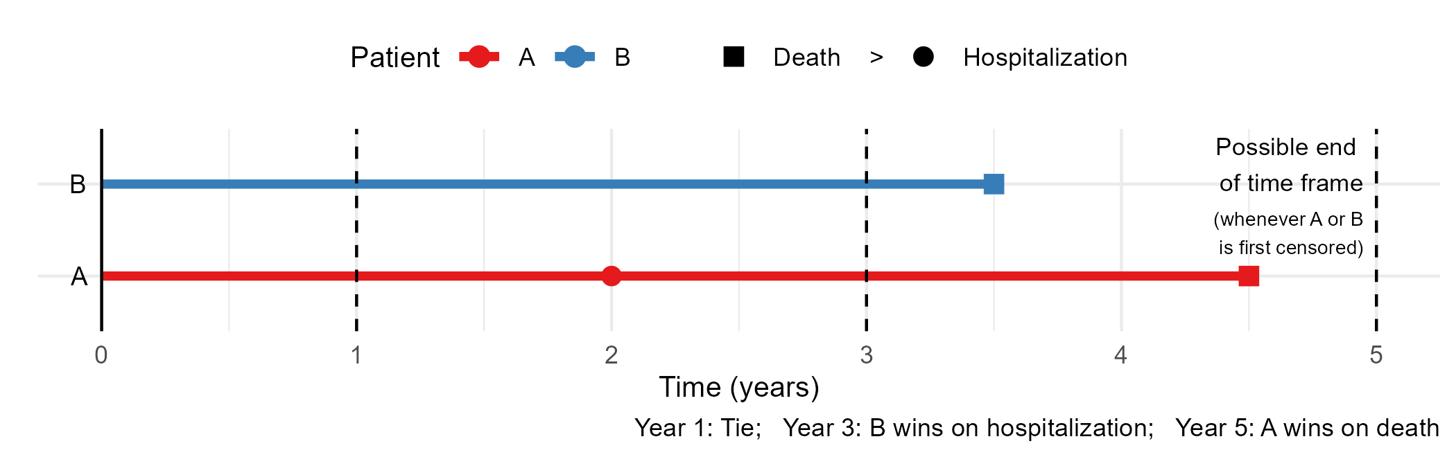
1.5 Win Ratio and Hierarchical Approaches
The win ratio (WR) offers a solution by comparing patient pairs across treatment arms. Each pair is evaluated hierarchically:
Longer survival indicates a win.
If both survive, fewer or later nonfatal events confer a win.
If tied, functional outcomes may be compared.
The win ratio is defined as: \[
\widehat{\text{WR}} = \frac{\text{\# of treatment wins}}{\text{\# of control wins}}.
\]
These measures align with clinical priorities and are increasingly used in practice.
1.6 Estimand Challenges
A critical limitation of the win ratio is its dependency on censoring. Because patients may be censored at different times, the win/loss status of a pair can change over time. The observed win ratio thus reflects an average over the censoring distribution, not a fixed population quantity.
This raises concerns for interpretation and estimation:
Testing remains valid under the null hypothesis, especially if the treatment consistently outperforms control.
Estimation, however, is biased unless a fixed follow-up time is defined or a model constrains the win ratio to be constant over time.
The ICH E9 (R1) addendum emphasizes that a clearly defined estimand is essential for interpreting treatment effects. For the win ratio, this requires careful attention to follow-up duration and censoring.
1.7 Toward Model-Based Estimands
Limitations of traditional and empirical approaches motivate model-based alternatives:
The restricted mean time in favor (RMT-IF) quantifies the net amount of time one group remains in a more favorable state.
The proportional win-fractions (PW) model expresses the win ratio as a function of covariates, enabling estimation of treatment effects under a semiparametric framework.
Both methods respect clinical hierarchies and avoid dependence on arbitrary censoring patterns. They form the foundation of the methods introduced in subsequent chapters.
1.8 Example R code
The following example assumes a data frame df in long format, with columns:
######################################### 1. Prepare data for survival analyses########################################library(dplyr)# For time-to-death analysis: remove nonfatal eventsdf_death <- df |>filter(status !=2)# For time-to-first-event (TFE): take earliest record per subjectdf_tfe <- df |>arrange(id, time) |>group_by(id) |>slice_head() |>ungroup()######################################### 2. Cox models for death and TFE########################################library(survival)# Time to deathcox_death <-coxph(Surv(time, status ==1) ~ trt, data = df_death)# Time to first event (death or nonfatal)cox_tfe <-coxph(Surv(time, status >0) ~ trt, data = df_tfe)######################################### 3. Weighted total events analysis########################################library(Wcompo)# Weighting: death:nonfatal = 2:1fit_wte <-CompoML(id, time, status, Z = trt, data = df, w =c(2, 1))
1.9 Conclusion
Standard methods for analyzing composite endpoints—such as time to first event or weighted event counts—often oversimplify patient trajectories and obscure clinically important effects. Hierarchical approaches like the win ratio offer a more principled alternative but require careful attention to the estimand, especially in the presence of censoring. Modern methods such as RMT-IF and the proportional win-fractions model provide robust and interpretable tools for analyzing composite outcomes in a way that respects both clinical priority and statistical rigor.