Statistical Methods for Composite Endpoints: Win Ratio and Beyond
Chapter 3 - Nonparametric Estimation
Department of Biostatistics & Medical Informatics
University of Wisconsin-Madison
May 31, 2025
Outline
Restricted win ratio
- WR estimand under fixed time frame (
WINSpackage)
- WR estimand under fixed time frame (
Restricted mean time in favor of treatment
- An extension of RMST
- HF-ACTION example (
rmtpackage)
While alive analysis of weighted total events
- Adjusts for duration of survival
- HF-ACTION example (
WApackage)
\[\newcommand{\d}{{\rm d}}\] \[\newcommand{\T}{{\rm T}}\] \[\newcommand{\dd}{{\rm d}}\] \[\newcommand{\cc}{{\rm c}}\] \[\newcommand{\pr}{{\rm pr}}\] \[\newcommand{\var}{{\rm var}}\] \[\newcommand{\se}{{\rm se}}\] \[\newcommand{\indep}{\perp \!\!\! \perp}\] \[\newcommand{\Pn}{n^{-1}\sum_{i=1}^n}\] \[ \newcommand\mymathop[1]{\mathop{\operatorname{#1}}} \] \[ \newcommand{\Ut}{{n \choose 2}^{-1}\sum_{i<j}\sum} \] \[ \def\a{{(a)}} \def\b{{(1-a)}} \def\t{{(1)}} \def\c{{(0)}} \def\d{{\rm d}} \def\T{{\rm T}} \def\bs{\boldsymbol} \]
Restricted Win Ratio
The Estimand Issue
- WR estimand depends on censoring
- Mixing different time frames \([0, C_i^\t\wedge C_j^\c]\) in win-loss calculations
- Censoring-weighted average of time-dependent win-loss (Ch 2) \[
\frac{\hat w_{1,0}}{\hat w_{0,1}}\to
\frac{\int_0^\infty\pr(\mbox{Treatment wins by } t)\dd G(t)}
{\int_0^\infty\pr(\mbox{Control wins by } t)\dd G(t)}
\]
- \(G(t)\): Distribution function of \(C^\t\wedge C^\c\)
- Trial-dependent; lacks generalizability
- Two ways to construct estimand (Ch 1)
- Pre-define restriction time
- Specify a time-constant WR model (Ch 4)
Time Restriction - Univariate
- Outcome data
- \(D^\a\): survival time for a patient in group \(a = 1, 0\)
- \(S^\a(t) = P(D^\a>t)\)
- \(D^\a\): survival time for a patient in group \(a = 1, 0\)
- Time restriction: a familiar concept
- Five-year survival rate of breast cancer patients
- Estimand: \(S^\t(\tau) - S^\c(\tau)\)
- Five-year average survival time
- Estimand: \(E\{\min(D^\t, \tau)\} - E\{\min(D^\c, \tau)\}\)
- Restricted mean survival time (RMST) (Tian et al., 2020)
- Restriction time \(\tau=5\) years (pre-specify)
- Five-year survival rate of breast cancer patients
Time Restriction - WR
- Two-tiered composite
- \(D^\a\): survival time; \(T_1^\a\): time to first nonfatal event
- Restricted win/loss probability
- Image all patients followed up to \(\tau\) \[\begin{align}\label{eq:wl_2comp} w_{a, 1-a}(\tau) &= \underbrace{\pr\{D^\b < \min(D^\a, \tau)\}}_{\mbox{win on survival}}\\ & + \underbrace{\pr\{\min(D^\t, D^\c) > \tau, T^\b < \min(T^\a, \tau)\}}_{\mbox{tie on survival, win on nonfatal event}} \end{align}\]
- Restricted (Pocock) WR: \({\rm WR}(\tau)=w_{1, 0}(\tau)/w_{0, 1}(\tau)\)
Estimation: IPCW or MI
- General win function
- Win/loss probability by \(t\) \[ w_{a, 1-a}(\tau)=\pr\left\{\mathcal W(\mathcal H^{*{(a)}}, \mathcal H^{*{(1-a)}})(\tau)=1\right\} \]
- Estimation: deal with data censored before \(\tau\)
- Inverse probability censoring weighting (IPCW, Dong et al., 2020b, 2021)
- R-package:
WINS(Cui & Huang, 2023)
- R-package:
- Multiple imputations (MI) for censored/missing data (Wang et al., 2023, 2024)
- Inverse probability censoring weighting (IPCW, Dong et al., 2020b, 2021)
RMT-IF
A Variation of RWR
- Take time difference into account
- \(w_{a, 1-a}(\tau)\): win probability by \(\tau\) \[ w_{1, 0}(\tau) - w_{0, 1}(\tau) = \mbox{Restricted proportional in favor (net benefit)} \]
- \(w_{a, 1-a}(\tau)\): re-define as average win time by \(\tau\) \[ w_{1, 0}(\tau) - w_{0, 1}(\tau) = \mbox{Restricted mean time in favor (RMT-IF)} \]
- RMT-IF
- Measures net average time treatment wins against control
- Convenient with multistate outcomes
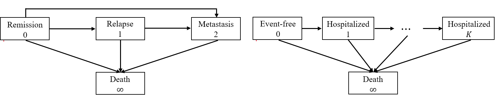
Multistate Outcomes
- Reformulate outcomes
- Multistate process: \(Y(t) \in \{0, 1,\ldots, K, \infty\}\)
- \(0\): initial state (e.g., remission, event-free)
- \(1, \ldots, K\): a series of progressively worse states
- \(\infty\): death
- Examples
- \(1\): relapse; \(2\): metastasis
- \(1, 2, \ldots\): cumulative number of hospitalizations
![]()
- Multistate process: \(Y(t) \in \{0, 1,\ldots, K, \infty\}\)
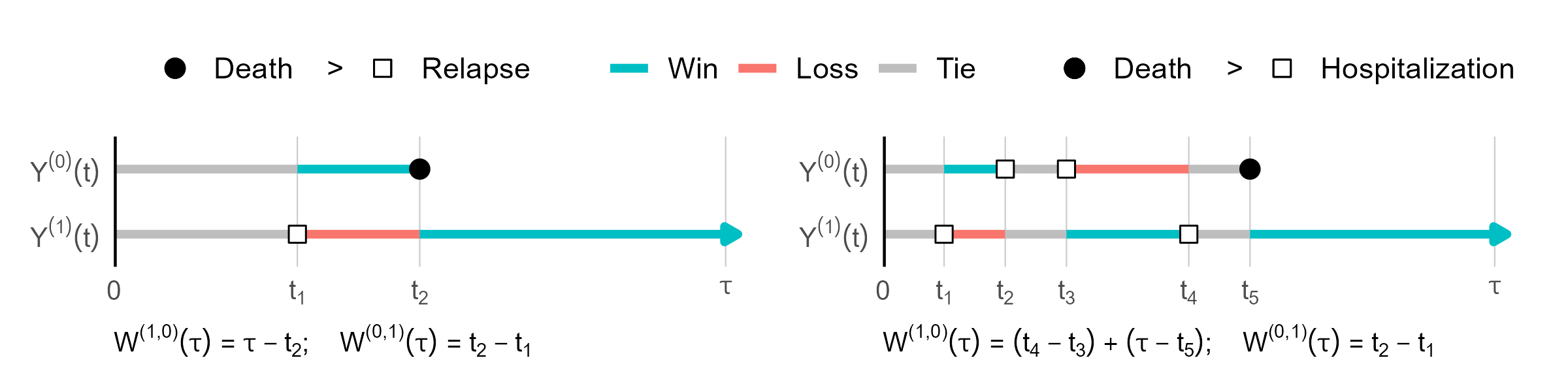
Time on a Win or Loss
- Pairwise win-loss time
- \(Y^\t(t)\) vs \(Y^\c(t)\) over \([0, \tau]\)
- Win time \(=\) time residing in a lower-tiered state \[
W^{(a, 1-a)}(\tau)=\int_0^\tau I\{Y^\a(t)<Y^\b(t)\}\d t
\]
![]()
Net Average Win Time
- Etimand of treatment effect
- RMT-IF of treatment (Mao, 2023b) \[
\mu(\tau) = w_{1, 0}(\tau) - w_{0, 1}(\tau)
\]
- Average win time: \(w_{a, 1-a}(\tau) = E\{W^{(a, 1-a)}(\tau)\}\)
- \(\mu(\tau)\): net average win time by treatment vs control
- Reduces to difference in RMST in life-death model
- Decomposition: Time won on which component?
- Extra survival time + extra relapse-free time + …
- RMT-IF of treatment (Mao, 2023b) \[
\mu(\tau) = w_{1, 0}(\tau) - w_{0, 1}(\tau)
\]
Decomposition
- Stage-wise effects \(\mu(\tau) = \sum_{k=1}^{K,\infty} \mu_k(\tau)\)
- Average win time on state \(k\) (being in a better state) \[w_{a, 1-a, k}(\tau)=E\left\{\int_0^\tau I\{Y^{(a)}(t)<Y^{(1-a)}(t) = k\}{\rm d}t\right\}\]
- Net average win time on state \(k\) \[
\mu_k(\tau)=w_{1, 0, k}(\tau) - w_{0, 1, k}(\tau)
\]
- \(\mu_\infty(\tau)\): net win time on survival \(=\) difference in \(\tau\)-RMST
- \(\mu_2(\tau)\): extra metastasis-free time; \(\mu_1(\tau)\): extra relapse-free time
- Further decomposition (Mao & Wang, 2024)
- \(\mu_k(\tau)=\sum_{j < k}\mu_{jk}(\tau)\): net average time improved from state \(k\) to state \(j\)
- \(\mu_\infty(\tau)=\mu_{0,\infty}(\tau)+ \mu_{1,\infty}(\tau)+\mu_{2,\infty}(\tau)\): net survival time in different states
Simplify for Progressive Processes
- Progressive process
- Definition: \(Y^{(a)}(t)\leq Y^{(a)}(s)\) for all \(0\leq t\leq s\)
- Only marching forward (all earlier examples)
- Transition time \(T_k^{(a)}\): time to transition to a state \(\geq k\)
- \(T_1^{(a)}\): time to relapse/metastasis/death
- \(T_2^{(a)}\): time to metastasis/death
- \(T_\infty^{(a)}=D^{(a)}\): time to death
- Reformulation: \(Y^{(a)}(\cdot)\equiv \big\{0\leq T_1^{(a)}\leq\cdots\leq T_K^{(a)}\leq T_\infty^{(a)}\big\}\)
- A progressive process \(\Longleftrightarrow\) a sequence of transition events
- Definition: \(Y^{(a)}(t)\leq Y^{(a)}(s)\) for all \(0\leq t\leq s\)
Delve into Estimand
- Average win time on state \(k\)
- Re-expression with \(S_k^{(a)}(t)=\pr\{T_k^{(a)}> t\}\) \[\begin{align} w_{a, 1-a, k}(\tau)&=\int_0^\tau \pr\{Y^{(a)}(t)< k\}\pr\{Y^{(1-a)}(t) = k\}{\rm d}t\\ &=\int_0^\tau \pr\{T_k^{(a)}> t\}\pr\{T_k^{(1-a)}\leq t < T_{k+1}^{(1-a)}\}{\rm d}t\\ &=\int_0^\tau S_k^{(a)}(t)\left\{S_{k+1}^{(1-a)}(t) - S_k^{(1-a)}(t)\right\}{\rm d}t\\ \end{align}\]
- Net average win time \[\mu_k(\tau)=w_{1, 0, k}(\tau)-w_{0, 1, k}(\tau)= \int_0^\tau \left\{S_k^{(1)}(t)S_{k+1}^{(0)}(t) - S_k^{(0)}(t)S_{k+1}^{(1)}(t)\right\}{\rm d}t\]
Observed Data & Estimation
- Censored observations
- \(Y(t\wedge C)\), or \[
(X_k^{(a)}, \delta_k^{(a)}),\,\,\, k =1,\ldots, K, \infty
\]
- \(X_k^{(a)}= \min(T_k^{(a)}, C^{(a)})\); \(\delta_k^{(a)}= I(T_k^{(a)}\leq C^{(a)})\); \(C^{(a)}=\) censoring time
- \(Y(t\wedge C)\), or \[
(X_k^{(a)}, \delta_k^{(a)}),\,\,\, k =1,\ldots, K, \infty
\]
- Estimation
- Plug-in KM estimator \(\hat S_k^{(a)}(t)\) \[ \hat\mu_k(\tau)= \int_0^\tau \left\{\hat S_k^{(1)}(t)\hat S_{k+1}^{(0)}(t) - \hat S_k^{(0)}(t)\hat S_{k+1}^{(1)}(t)\right\}{\rm d}t \]
- Robust variance estimator for \(\hat\mu_k(\tau)\)
Hypothesis Testing
- Test of overall effect
- \(\chi_1^2\) test based on \(\hat\mu(\tau)=\sum_{k=1}^{K,\infty}\hat\mu_k(\tau)\) for \[ H_0: \mu(\tau)= 0 \]
- Joint test on components
- \(\chi_{K+1}^2\) test based on \(\hat\mu_1(\tau),\ldots,\hat\mu_K(\tau),\hat\mu_\infty(\tau)\) \[
H_0: \mu_1(\tau)=\cdots=\mu_K(\tau)=\mu_\infty(\tau)
\]
- May be more powerful under differential component-wise effects
- Test individual components for secondary analyses
- \(\chi_{K+1}^2\) test based on \(\hat\mu_1(\tau),\ldots,\hat\mu_K(\tau),\hat\mu_\infty(\tau)\) \[
H_0: \mu_1(\tau)=\cdots=\mu_K(\tau)=\mu_\infty(\tau)
\]
Sample Size Calculation
- Bivariate illness-death
- Gumbel–Hougaard copula (Mao, 2023c)
- Same model used for sample size calculation for WR
- Input parameters
- Baseline: Hazards for death & relapse, association parameter
- Effect sizes: Component-wise hazard ratios
- Gumbel–Hougaard copula (Mao, 2023c)
- Recurrent events with death
- Homogeneous Markov model (Mao, 2023d)
- Input parameters
- Baseline: Intensities for another hospitalization or death, having had \(k-1\) hospitalizations \((k=1,2,\ldots)\)
- Effect sizes: Intensity (risk) ratios for all transitions
Software: rmt::rmtfit() (I)
- Input data format (long)
- Standard multistate
status = kfor entry into state \(k\),K+1for death,0for censoring
- Recurrent events with death
status = 1for nonfatal event,2for death,0for censoring
- Standard multistate
Software: rmt::rmtfit() (II)
- Basic syntax
- Output: a list of class
rmtfitobj$t: \(t\);obj$mu: a matrix of \((K+2)\) rows, \(\hat\mu_k(t)\) in \(k\)th row, \(\hat\mu(t)\) in last;obj$var: variances of point estimates inmusummary(obj, tau)for summary results on \(\mu(\tau)\), including the \(\mu_k(\tau)\)- Recurrent events: specify
Kmax = kto merge \(\mu_{k+}(\tau)\sum_{k'=k}^K=\mu_{k'}(\tau)\)
- Recurrent events: specify
plot(obj)to plot \(\hat\mu(t)\) against \(t\)
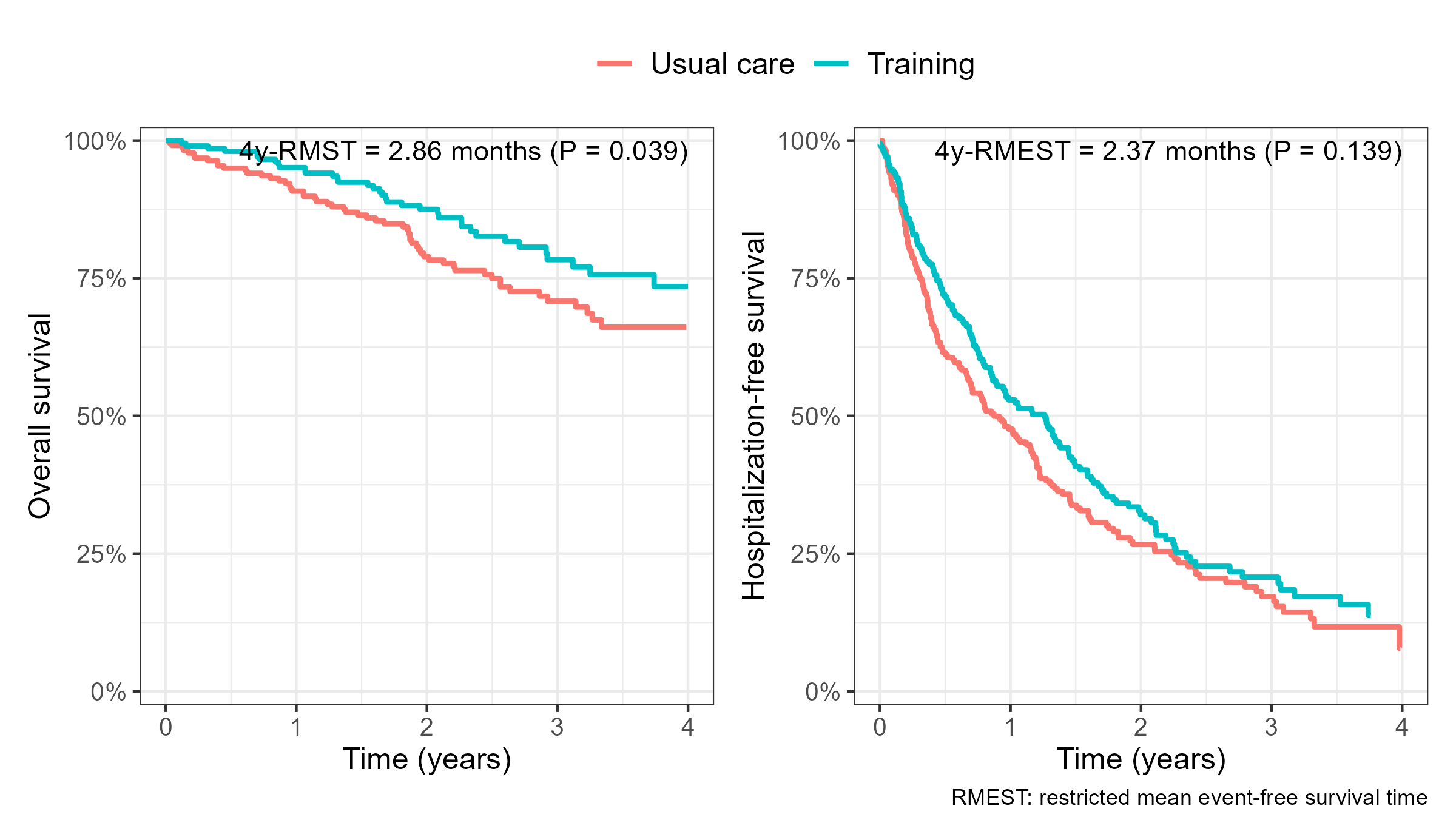
HF-ACTION: Standard Analyses
- Traditional composite and overall survival
![]()
R-Code
- Fit 4y-RMT-IF
obj <- rmtfit(hfaction$patid, hfaction$time, hfaction$status, hfaction$trt_ab,
type = "recurrent")
summary(obj, Kmax = 4, tau = 3.97) ## combine recurrent events >= 4
# Restricted mean time in favor of group "1" by time tau = 3.97:
# Estimate Std.Err Z value Pr(>|z|)
# Event 1 0.0140515 0.0498836 0.2817 0.778184
# Event 2 0.0358028 0.0499618 0.7166 0.473619
# Event 3 0.1385287 0.0409533 3.3826 0.000718 ***
# Event 4+ -0.0064731 0.0600813 -0.1077 0.914203
# Survival 0.2384169 0.1143484 2.0850 0.037069 *
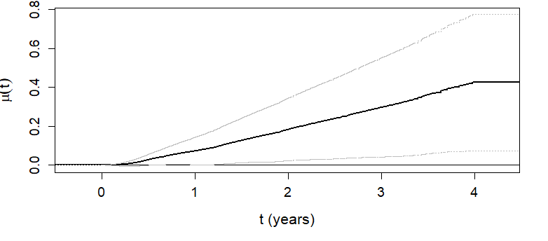
# Overall 0.4203268 0.1777363 2.3649 0.018035 * Graphics
\(\hat\mu(t)\) as a function of \(t\)
- Overall RMT-IF becomes significant after 1 year (see lower CL)
![]()
Inference Results
- 4-year RMT-IF of exercise training
- Training on average gains 5.1 months (\(P\)=0.018) in favorable state
- 2.9 months net survival \(+\) 2.2 months net time with fewer hosps (little effect on 1st)
- Training on average gains 5.1 months (\(P\)=0.018) in favorable state
| Estimate | SE | P-value | ||
|---|---|---|---|---|
| Hopitalization | 2.18 | 1.22 | 0.073 | |
| 1 | 0.17 | 0.60 | 0.778 | |
| 2 | 0.43 | 0.60 | 0.474 | |
| 3 | 1.66 | 0.49 | <0.001 | |
| 4+ | -0.08 | 0.72 | 0.914 | |
| Death | 2.86 | 1.37 | 0.037 | |
| Overall | 5.04 | 2.13 | 0.018 |
While-Alive Weighted Loss
Length of Exposure
- HF-ACTION
- Trained survive longer \(\to\) more hospitalizations
| Usual care (N = 221) | Exercise training (N = 205) | |
|---|---|---|
| Death | 57 (25.8%) | 36 (17.6%) |
| Avg # hospitalization (SD) | 2.6 (3.1) | 2.2 (3.1) |
- Impact of differential survival time
- Hierarchical: WR, RMT-IF (death > nonfatal)
- Hospitalizations considered only with tied (equal) survival
- Quantitative weighting: cumulative mean (death = \(w_D\times\) nonfatal; Ch 1)
- Need to adjust for length of exposure (survival)
- Hierarchical: WR, RMT-IF (death > nonfatal)
Weighted Endpoints
- Weighted composite event process (Ch 1)
- \(N^{*\a}_{\rm R}(t)=w_DN^{*\a}_D(t)+\sum_{k=1}^Kw_kN^{*\a}_k(t)\)
- \({\rm d}N_{\rm R}^{*(a)}(t)=0\) for \(t>D^{(a)}\): no event after death
![]()
- \({\rm d}N_{\rm R}^{*(a)}(t)=0\) for \(t>D^{(a)}\): no event after death
- \(N^{*\a}_{\rm R}(t)=w_DN^{*\a}_D(t)+\sum_{k=1}^Kw_kN^{*\a}_k(t)\)
- Traditional methods
- Cause-specific rate (death as censoring): \(E\left\{{\rm d}N_{\rm R}^{*(a)}(t)\mid D^{(a)}\geq t\right\}\)
- Lacking in causal interpretation: \(\left\{\cdot\mid D^\t\geq t\right\}\) vs \(\left\{\cdot\mid D^\c\geq t\right\}\) at post-randomization \(t\)
- Cumulative mean: \(E\left\{N_{\rm R}^{*(a)}(t)\right\}\) (Ghosh & Lin, 2000; Mao & Lin, 2016)
- Ignores length of exposure
- Cause-specific rate (death as censoring): \(E\left\{{\rm d}N_{\rm R}^{*(a)}(t)\mid D^{(a)}\geq t\right\}\)

Exposure-Adjusted Rate
- While-alive event rate
- Estimand \[\ell^{(a)}(\tau) = \frac{E\left\{N_{\rm R}^{*(a)}(\tau)\right\}}{E\left(D^{(a)}\wedge\tau\right)} =\frac{\mbox{Mean # of weighted events by $\tau$}}{\mbox{Mean survival time by $\tau$}} \]
- Average (weighted) event rate in \([0, \tau]\) per person-time alive
- Proposed as a clinically interpretable measure to Committee for Medicinal Products for Human Use (CHMP) of European Medicines Agency (Akacha et al., 2018; CHMP, 2020)
- Also called “exposure-weighted” event rate
General Estimands: Definition
- While-alive loss rate
- Estimand (Mao, 2023a) \[\ell^{(a)}(\tau) = \frac{E\left\{\mathcal L\left(\mathcal H^{*(a)}\right)(\tau)\right\}}{E\left(D^{(a)}\wedge\tau\right)}\]
- \(\mathcal H^{*{(a)}}(t)=\left\{N^{*{(a)}}_D(u), N^{*{(a)}}_1(u), \ldots, N^{*{(a)}}_K(u):0\leq u\leq t\right\}\)
- \(\mathcal L\left(\mathcal H^{*(a)}\right)(t)\): user-specified loss function satisfying
- A function only of \(\mathcal H^{(a)}(t)\)
- \(\mathcal L\left(\mathcal H^{*(a)}\right)({\rm d}t)\equiv 0\) for \(t>D^{(a)}\) (accrue loss only when alive)
- Average loss rate in \([0, \tau]\) per person-time alive
- Estimand (Mao, 2023a) \[\ell^{(a)}(\tau) = \frac{E\left\{\mathcal L\left(\mathcal H^{*(a)}\right)(\tau)\right\}}{E\left(D^{(a)}\wedge\tau\right)}\]
General Estimands: Examples
- Difference choices of loss function
- Original while-alive event rate \[\mathcal L\left(\mathcal H^{*(a)}\right)(t) = N_{\rm R}^{*(a)}(t)\]
- Per-person-time mortality rate (Uno & Horiguchi, 2023) \[\mathcal L\left(\mathcal H^{*(a)}\right)(t) = N_D^{*(a)}(t)\]
- More generally… \[\mathcal L\left(\mathcal H^{*(a)}\right)(t)
= \int_0^t \left\{w_{D, N^{*(a)}(u-)}(u)\dd N^{*\a}_D(t)+\sum_{k=1}^Kw_{k, N^{*(a)}(u-)}(u)\dd N^{*\a}_k(t)\right\}\]
- \(w_{D,m}(u), w_{k,m}(u)\): weights for incident death/nonfatal events at \(u\) with \(m\) existing events
Cumulative and Differentials
- Cumulative version
- Survival-completed cumulative loss \[L^{(a)}(\tau)=\ell^{(a)}(\tau)\tau\]
- Better graphics: \(\ell^{(a)}(\tau)\approx 0/0\) unstable for \(\tau\approx 0\)
- Properties: \(L^{(a)}(0)=0\), \(L^{(a)}(t)\uparrow\) with \(t\), and \(L^{(a)}(t)\geq E\{\mathcal L(\mathcal H^{(a)})(t)\}\)
- Survival-completed cumulative loss \[L^{(a)}(\tau)=\ell^{(a)}(\tau)\tau\]
- Measuring treatment effect
- Risk (loss rate) ratio (RR): \(r(\tau)=\ell^{(1)}(\tau)/\ell^{(0)}(\tau)\)
- Treatment reduces average loss rate by \(100\{1-r(\tau)\}\%\)
- Absolute risk reduction: \(d(\tau)=\ell^{(1)}(\tau)-\ell^{(0)}(\tau)\)
- Treatment reduces average loss rate by \(-d(\tau)\) (per person-time alive)
- Risk (loss rate) ratio (RR): \(r(\tau)=\ell^{(1)}(\tau)/\ell^{(0)}(\tau)\)
Nonparametric Estimation
- With patients censored before \(\tau\)
Sample averages for numerator/denominator\[\ell^{(a)}(\tau) = \frac{E\left\{\mathcal L\left(\mathcal H^{*(a)}\right)(\tau)\right\}}{E\left(D^{(a)}\wedge\tau\right)}\]- Denominator (easy): RMST \(=\int_0^\tau S^{(a)}(t){\rm d}t\) (Royston & Parmar, 2011)
- Plug-in KM estimator
- Numerator (moderate) \(=\int_0^\tau S^{(a)}(t-)E\{\mathcal L(\mathcal H^{(a)})({\rm d}t)\mid D^{(a)}\geq t\}\)
- Nelsen-Aalen-type estimator for \(E\{\mathcal L(\mathcal H^{(a)})({\rm d}t)\mid D^{(a)}\geq t\}\)
- Robust variance estimation
- Implementation in
WApackage
Software: WA::LRfit()
- Basic syntax
id: unique patient identifier;time: event times;status: event types (1: recurrent event,2: death,0: censoring)Dweight: weight for death relative to nonfatal
- Output: a list of class
LRfitsummary(obj, tau)to summarize results for \(r(\tau)=\ell^{(1)}(\tau)/\ell^{(0)}(\tau)\)- Add
joint.test = TRUEto include joint test with RMST
- Add
plot(obj)to plot the cumulative (WA) loss \(L^\a(t)\) (\(a= 1, 0\))
HF-ACTION: Weighted Composite
- 4y-loss rate (death = \(2\times\) hosp)
- Risk ratio: \(79.8\%\) (\(P=0.102\)) reduction in risk
- cf. Cumulative mean ratio (unadjusted): 85.7% (\(P=0.170\)) (Ch 1)
- Risk ratio: \(79.8\%\) (\(P=0.102\)) reduction in risk
obj <- LRfit(hfaction$patid, hfaction$time, hfaction$status,
hfaction$trt_ab, Dweight = 2)
summary(obj, tau = 3.97)
# Analysis of log loss rate (LR) by tau = 3.97:
# Estimate Std.Err Z value Pr(>|z|)
# Ref (Group 0) 0.262765 0.086018 3.0548 0.002252 **
# Group 1 vs 0 -0.226116 0.138131 -1.6370 0.101637
# ---
# Signif. codes: 0 ‘***’ 0.001 ‘**’ 0.01 ‘*’ 0.05 ‘.’ 0.1 ‘ ’ 1
# Point and interval estimates for the LR ratio:
# LR ratio 95% lower CL 95% higher CL
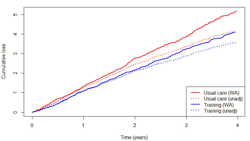
# Group 1 vs 0 0.7976253 0.6084453 1.045626HF-ACTION: Survival Adjustment
- Survival-adjusted vs unadjusted cumulative loss
- Unadjusted shows attenuated effect
![]()
- Unadjusted shows attenuated effect
Conclusion
Notes
- Analysis of win-loss times
- Variations including RMT-IF in comparison with WR (Troendle et al., 2024)
- While-alive estimands
- Papers following CHMP discussion (Fritsch et al., 2023; Schmidli et al., 2023a, 2023b; Wei et al., 2023)…
- RMT-IF vs WA in HF-ACTION
- RMT-IF appears more powerful \(\to\) adds significance to mortality alone
- \(P=0.037 \to 0.018\)
- WA still sees a dilution of effect
- \(P=0.033 \to 0.102\)
- RMT-IF appears more powerful \(\to\) adds significance to mortality alone
Summary
Nonparametric estimands by time restriction
- Restricted WR
- WR on all patients followed to \(\tau\)
- IPCW (
WINS) or MI
- IPCW (
- WR on all patients followed to \(\tau\)
- RMT-IF
- Net average win time on hierarchical states by \(\tau\)
rmt::rmtfit(id, time, status, trt)
- Net average win time on hierarchical states by \(\tau\)
- While-alive weighted events
- Compensate for differential survival by \(\tau\)
WA::LRfit(id, time, status, trt, Dweight)
- Compensate for differential survival by \(\tau\)