Statistical Methods for Composite Endpoints: Win Ratio and Beyond
Chapter 2 - Hypothesis Testing
Department of Biostatistics & Medical Informatics
University of Wisconsin-Madison
May 31, 2025
Outline
- Win ratio basics and properties
- Generalize to recurrent events
- HF-ACTION example (
WRpackage)
- HF-ACTION example (
- Sample size calculations
- HF-ACTION example (
WRpackage) \[\newcommand{\d}{{\rm d}}\] \[\newcommand{\T}{{\rm T}}\] \[\newcommand{\dd}{{\rm d}}\] \[\newcommand{\cc}{{\rm c}}\] \[\newcommand{\pr}{{\rm pr}}\] \[\newcommand{\var}{{\rm var}}\] \[\newcommand{\se}{{\rm se}}\] \[\newcommand{\indep}{\perp \!\!\! \perp}\] \[\newcommand{\Pn}{n^{-1}\sum_{i=1}^n}\] \[ \newcommand\mymathop[1]{\mathop{\operatorname{#1}}} \] \[ \newcommand{\Ut}{{n \choose 2}^{-1}\sum_{i<j}\sum} \] \[ \def\a{{(a)}} \def\b{{(1-a)}} \def\t{{(1)}} \def\c{{(0)}} \def\d{{\rm d}} \def\T{{\rm T}} \def\bs{\boldsymbol} \]
- HF-ACTION example (
Win Ratio Basics & Properties
Standard Two-Sample
- Two-sample comparison (Pocock et al., 2012)
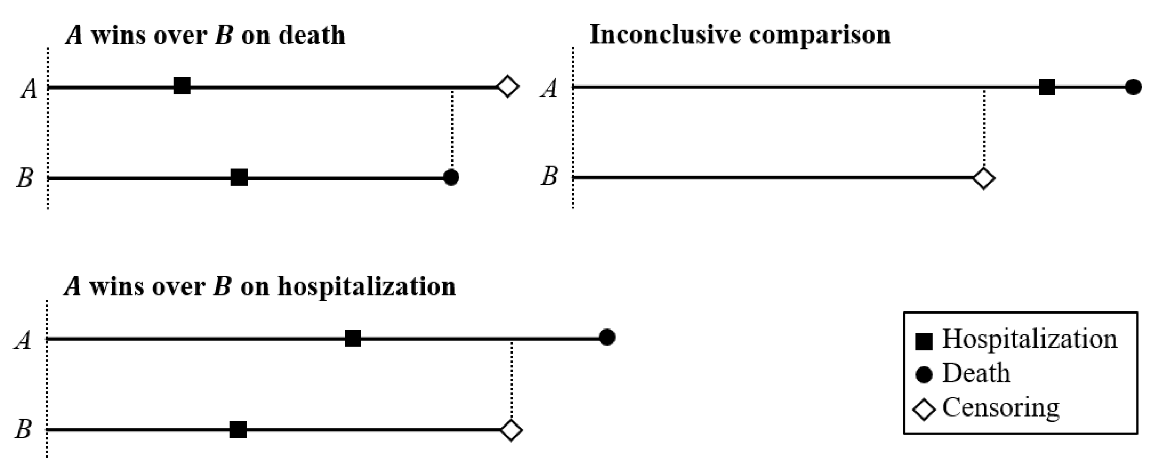
- Data: \(D_i^{(a)}, T_i^{(a)}, C_i^{(a)}\): survival, hospitalization, censoring times on \(i\)th subject in group \(a\) \((i=1,\ldots, N_a; a= 1, 0)\)
- Pairwise comparisons: \(i\)th in group \(a\) vs \(j\)th in group \(1-a\)
- Hierarchical composite: Death > hospitalization in \(\left[0, C_i^{(a)}\wedge C_j^{(1-a)}\right]\) \[\begin{align} \hat w^{(a, 1-a)}_{ij}&= \underbrace{I(D_j^{(1-a)}< D_i^{(a)}\wedge C_i^{(a)}\wedge C_j^{(1-a)})}_{\mbox{win on survival}}\\ & + \underbrace{I(\min(D_i^{(a)}, D_j^{(1-a)}) > C_i^{(a)}\wedge C_j^{(1-a)}, T_j^{(1-a)}< T_i^{(a)}\wedge C_i^{(1)}\wedge C_j^{(0)})}_{\mbox{tie on survival, win on hospitalization}} \end{align}\]
Pocock’s Rule
- Win, lose, or tie?
Calculation of Win Ratio
- Two-sample statistics
- Win (loss) fraction for group \(a\) (\(1-a\)) \[ \hat w^{(a, 1-a)}=(N_0N_1)^{-1}\sum_{i=1}^{N_a}\sum_{j=1}^{N_{1-a}}\hat w^{(a, 1-a)}_{ij}\]
- Win ratio statistic \[ WR = \hat w^{(1, 0)} / \hat w^{(0, 1)} \]
- Other measures
- Net benefit (proportion in favor): \(\hat w^{(1, 0)} - \hat w^{(0, 1)}\) (Buyse, 2010)
- Win odds: \((\hat w^{(1, 0)} - \hat w^{(0, 1)} + 1)/ (\hat w^{(0, 1)} - \hat w^{(1, 0)} + 1)\) (Dong et al., 2020)
The Binary Case
- Consider binary \(Y^{(a)}= 1, 0\)
- \(\hat w^{(a, 1-a)}_{ij} = I(Y_i^{(a)}> Y_j^{(1-a)})=Y_i^{(a)}(1-Y_j^{(1-a)})\)
- Win (loss) fraction \[
\hat w^{(a, 1-a)} = (N_1N_0)^{-1}\sum_{i=1}^{N_a}\sum_{j=1}^{N_{1-a}}Y_i^{(a)}(1-Y_j^{(1-a)})
= \hat p^{(a)}(1-\hat p^{(1-a)})\]
- \(\hat p^{(a)}= N_a^{-1}\sum_{i=1}^{N_a} Y_i^{(a)}\) (success probability)
- Equivalencies \[\begin{align} {\rm Win\,\, ratio}&= \frac{\hat w^{(1, 0)}}{\hat w^{(0, 1)}} = \frac{\hat p^{(1)}(1-\hat p^{(0)})}{\hat p^{(0)}(1-\hat p^{(1)})} = {\rm Odds \,\, ratio}\\ {\rm Net \,\, benefit}&=\hat w^{(1, 0)} - \hat w^{(0, 1)} = \hat p^{(1)}- \hat p^{(0)}= {\rm Risk \,\, difference} \end{align}\]
Hypothesis Testing
- Test statistic
- Log-transformed and normalized \[
S_n = \frac{n^{1/2}\log(\hat w_{1,0}/\hat w_{0,1})}{\hat{\rm SE}} \stackrel{H_0}{\sim} N (0, 1)
\]
- \(\hat{\rm SE}\): standard error of numerator by \(U\)-statistic method (Bebu & Lachin, 2016; Dong et al., 2016; Luo et al., 2015); \(n = N_1 + N_0\)
- Null hypothesis \[
H_0: H^\t(s, t) = H^\c(s, t)\mbox{ for all } t\leq s
\]
- \(H^\a(s, t)=\pr(D^\a > s, T^\a > t)\)
- Log-transformed and normalized \[
S_n = \frac{n^{1/2}\log(\hat w_{1,0}/\hat w_{0,1})}{\hat{\rm SE}} \stackrel{H_0}{\sim} N (0, 1)
\]
Alternative Hypothesis
- What is estimand of WR?
- Censoring-weighted average of time-dependent WRs (Oakes, 2016) \[
\frac{\hat w_{1,0}}{\hat w_{0,1}}\to
\frac{\int_0^\infty\pr(\mbox{Treatment wins by } t)\dd G(t)}
{\int_0^\infty\pr(\mbox{Control wins by } t)\dd G(t)} =\text{Non-centrality parameter}
\]
- \(G(t)\): Distribution function of \(C^\t\wedge C^\c\)
- Treatment wins consistently against control over time (Mao, 2019) \[ H_A: \pr(\mbox{Treatment wins by } t)\geq \pr(\mbox{Control wins by } t) \mbox{ for all } t \]
- Sufficient condition: joint stochastic order of death and nonfatal event \[ H_A: H^\t(s, t) \geq H^\c(s, t)\mbox{ for all } t\leq s \]
- Censoring-weighted average of time-dependent WRs (Oakes, 2016) \[
\frac{\hat w_{1,0}}{\hat w_{0,1}}\to
\frac{\int_0^\infty\pr(\mbox{Treatment wins by } t)\dd G(t)}
{\int_0^\infty\pr(\mbox{Control wins by } t)\dd G(t)} =\text{Non-centrality parameter}
\]
Variations
Weighting
- Unweighted pairwise comparisons \(\to\) Gehan (1965) test
- Weight win/loss by time of follow-up \(\to\) log-rank (more efficient) (Luo et al., 2017)
Stratification
- Stratified WR: within-stratum comparisons (Dong et al., 2017, 2023; Gasparyan et al., 2020)
- Sum of stratum-specific wins / sum of stratum-specific losses
- Adjust for confounding; increase efficiency
- Stratified WR: within-stratum comparisons (Dong et al., 2017, 2023; Gasparyan et al., 2020)
Handling Recurrent Events
General Data
- Full outcomes
- A subject in group \(a\) \((a=1, 0)\) \[\mathcal H^{*{(a)}}(t)=\left\{N^{*{(a)}}_D(u), N^{*{(a)}}_1(u), \ldots, N^{*{(a)}}_K(u):0\leq u\leq t\right\}\]
- \(N^{*{(a)}}_D(u), N^{*{(a)}}_1(u), \ldots, N^{*{(a)}}_K(u)\): counting processes for death and \(K\) different types of nonfatal events
- Observed data
- \(\mathcal H^{*{(a)}}(X^{(a)})\): life history up to \(X^{(a)}= D^{(a)}\wedge C^{(a)}\)
General Rule of Comparison
- Win function
Time frame of comparison: \([0, t]\) \[\mathcal W(\mathcal H^{*{(a)}}, \mathcal H^{*{(1-a)}})(t) =I\left\{\mathcal H^{*{(a)}}(t) \mbox{ is more favorable than } \mathcal H^{*{(1-a)}}(t)\right\}\]
Basic requirements
- (W1) \(\mathcal W(\mathcal H^{*{(a)}}, \mathcal H^{*{(1-a)}})(t)\) is a function only of \(\mathcal H^{*{(a)}}(t)\) and \(\mathcal H^{*{(1-a)}}(t)\)
- (W2) \(\mathcal W(\mathcal H^{*{(a)}}, \mathcal H^{*{(1-a)}})(t)+\mathcal W(\mathcal H^{*{(1-a)}}, \mathcal H^{*{(a)}})(t) \in \{0, 1\}\)
- (W3) \(\mathcal W(\mathcal H^{*{(a)}}, \mathcal H^{*{(1-a)}})(t)=\mathcal W(\mathcal H^{*{(a)}}, \mathcal H^{*{(1-a)}})(D^{(a)}\wedge D^{(1-a)}\wedge t)\)
Interpretations
- (W1) Consistency of time frame
- (W2) Either win, loss, or tie
- (W3) No change of win-loss status after death (satisfied if death is prioritized)
Generalized Win Ratio
- Under general win function \(\mathcal W(\cdot,\cdot)\)
- Win ratio statistic \[\begin{equation}\label{eq:wr:gen_WR} \hat{\mathcal E}_n(\mathcal W)=\frac{(N_1N_0)^{-1}\sum_{i=1}^{N_1}\sum_{j=1}^{N_0}\mathcal W(\mathcal H^{*{(1)}}_{i}, \mathcal H^{*{(0)}}_{j})(X^{{(1)}}_{i}\wedge X^{{(0)}}_{j})} {(N_1N_0)^{-1}\sum_{i=1}^{N_1}\sum_{j=1}^{N_0}\mathcal W(\mathcal H^{*{(0)}}_{j}, \mathcal H^{*{(1)}}_{i})(X^{{(1)}}_{i}\wedge X^{{(0)}}_{j})} \end{equation}\]
- Still each pair is compared over \(\left[0, X^{{(1)}}_{i}\wedge X^{{(0)}}_{j}\right]\), but by a general rule \(\mathcal W\)
- Stratified win ratio: ratio between weighted sum of within-stratum win/loss fractions
Examples
- Pocock’s WR
- \(T^{(a)}_1\): time of first event in \(N^{*{(a)}}(t)=\sum_{k=1}^K N^{*{(a)}}_k(t)\) \[\begin{align}\label{eq:wr:PWR} \mathcal W_{\rm P}(\mathcal H^{*{(a)}}, \mathcal H^{*{(1-a)}})(t)&=I\{D^{(1-a)}<D^{(a)}\wedge t\}\notag\\ &\hspace{2mm}+I\{D^{(a)}\wedge D^{(1-a)}>t, T_{1}^{(1-a)}<T_{1}^{(a)}\wedge t\} \end{align}\]
- \(\hat{\mathcal E}_n(\mathcal W_{\rm P})\)
- TFE WR
- \(\tilde T^{(a)}=\min(D^{(a)}, T_1^{(a)})\) \[ \mathcal W_{\rm TFE}(\mathcal H^{*{(a)}},\mathcal H^{*{(1-a)}})(t)=I(\tilde T^{(1-a)}<\tilde T^{(a)}\wedge t) \]
- \(\hat{\mathcal E}_n(\mathcal W_{\rm TFE})\): allowable but not desirable
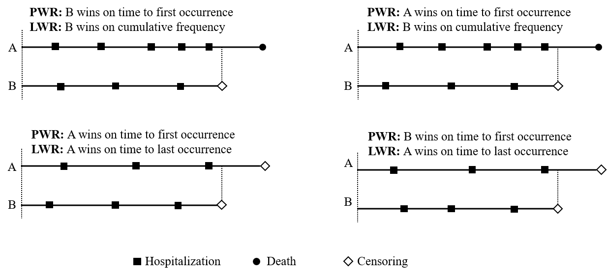
Options for Recurrent Events
- Three variations (Mao et al., 2022)
- Naive: Death > number of events (Finkelstein & Schoenfeld, 1999)
- First-event: Death > number of events > time to first event
- Last-event: Death > number of events > time to last event
- Properties
First/Last-event fewer ties than standard WR
First/Last-event \(\to\) Pocock’s WR with nonrecurrent event
Exercise
Write out the win function \(\mathcal W\) for the three versions of recurrent-event WR.
Comparison with Pocock’s
- Last-event WR (LWR)
- vs Pocock’s WR (PWR)
Alternative Hypothesis for LWR
- LWR
- Tests joint stochastic order of all events \[
H_A: H^\t(s, t_1, t_2, \ldots) \geq H^\c(s, t_1, t_2, \ldots)\mbox{ for all }
t_1\leq t_2\leq\cdots\leq s
\]
- \(H^\t(s, t_1, t_2, \ldots)=\pr(D^\a > s, T_1^\a > t_1, T_2^\a > t_2, \ldots)\)
- \(T_k^\a\): \(k\)th recurrent event in \(N^{*{(a)}}(t)\) \((k=1, 2, \ldots)\)
- Treatment stochastically delays all events
- All variations of WR implemented in
WRpackage- Simulations show LWR more powerful than rest (Mao et al., 2022)
- Tests joint stochastic order of all events \[
H_A: H^\t(s, t_1, t_2, \ldots) \geq H^\c(s, t_1, t_2, \ldots)\mbox{ for all }
t_1\leq t_2\leq\cdots\leq s
\]
Software: WR::WRrec()
- Basic syntax
- Long format
ID: unique patient identifier;time: event times;status: event types (1: death;2: recurrent events;0: censoring);trt: binary treatment;strata: strata variable naive = TRUE: calculates naive/FWR as well as LWR
- Long format
- Output: a list of class
WRrecobj$log.WR: log-LWR;obj$se: \(\hat\se(\mbox{log-LWR})\)print(obj)to print summary results
HF-ACTION: Data
High-risk subset \((n=426)\)
age60: indicator of age \(\geq\) 60 yrs
library(WR)
##### Read in HF-ACTION DATA########
# same as rmt::hfaction used in chap 1
#  (except for status coding)
data(hfaction_cpx9)
hfaction <- hfaction_cpx9
head(hfaction)
#>        patid       time status trt_ab age60
#> 1 HFACT00001  7.2459016      2      0     1
#> 2 HFACT00001 12.5573770      0      0     1
#> 3 HFACT00002  0.7540984      2      0     1
#> 4 HFACT00002  4.2950820      2      0     1
#> 5 HFACT00002  4.7540984      2      0     1
#> 6 HFACT00002 45.9016393      0      0     1
HF-ACTION: Summary
- Descriptive
| Usual care (N = 221) | Exercise training (N = 205) | ||
|---|---|---|---|
| Age | ≤ 60 years | 122 (55.2%) | 128 (62.4%) |
| > 60 years | 99 (44.8%) | 77 (37.6%) | |
| Follow-up | (months) | 28.6 (18.4, 39.3) | 27.6 (19, 40.2) |
| Death | 57 (25.8%) | 36 (17.6%) | |
| Hospitalizations | 0 | 51 (23.1%) | 60 (29.3%) |
| 1-3 | 114 (51.6%) | 102 (49.8%) | |
| 4-10 | 49 (22.2%) | 39 (19%) | |
| >10 | 7 (3.2%) | 4 (2%) |
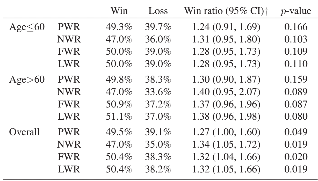
HF-ACTION: WR Analyses
Naive (NWR), first-event (FWR), LWR
- Stratified by age \(<\) or \(\geq 60\)
obj
#>             N Rec. Event Death Med. Follow-up
#> Control   221        571    57       28.62295
#> Treatment 205        451    36       27.57377
#>
#> WR analyses:
#>     Win prob Loss prob WR (95% CI)*      p-value
#> LWR 50.4%    38.2%     1.32 (1.05, 1.66) 0.0189
#> FWR 50.4%    38.3%     1.32 (1.04, 1.66) 0.0202
#> NWR 47%      35%       1.34 (1.05, 1.72) 0.0193
#> -----
#> *Note: The scale of WR depends on censoring distribution.
HF-ACTION: Overall
- Recurrent-event WRs more powerful than PWR
- NWR/FWR/LWR similar as \(N\) hosp is highly variable (0 - 26)
Sample Size Calculations
Special Case: PWR
- Simplified outcome model
- Gumbel-Hougaard copula (Oakes, 1989) \[
\pr(D^\a>s, T_1^\a>t) = \exp\left(-\left[\{\exp(a\xi_D)\lambda_Ds\}^\kappa + \{\exp(a\xi_H)\lambda_Ht\}^\kappa \right]^{1/\kappa}\right)
\]
- \(\lambda_D, \lambda_H\): baseline hazard rates for death/nonfatal event
- \(\exp(\xi_D), \exp(\xi_H)\): treatment HR on death/nonfatal event (effect sizes)
- \(\kappa\geq 1\): association parameter (Kendall’s rank correlation \(1-\kappa^{-1}\))
- Gumbel-Hougaard copula (Oakes, 1989) \[
\pr(D^\a>s, T_1^\a>t) = \exp\left(-\left[\{\exp(a\xi_D)\lambda_Ds\}^\kappa + \{\exp(a\xi_H)\lambda_Ht\}^\kappa \right]^{1/\kappa}\right)
\]
- Study design
- Uniform patient accrual over \([0, \tau_b]\); follow all until \(\tau>\tau_b\)
- Random loss-to-follow-up (LTFU) rate \(\lambda_L\)
Sample Size Formula
- Total sample size needed \[
n = \frac{\zeta_0^2(\lambda_D,\lambda_H,\kappa,\tau_c,\tau,\lambda_L)(z_{1-\alpha/2} + z_\gamma)^2}
{q(1-q)\delta(\lambda_D,\lambda_H,\kappa,\tau_c,\tau,\lambda_L)^\T\xi}
\]
- \(\alpha =0.05\): type I error; \(\gamma = 0.8, 0.9\): desired power (\(z_\gamma=\Phi^{-1}(\gamma)\))
- \(\xi=(\xi_D,\xi_H)^\T\): component-wise log-HRs (effect sizes)
- \(q=N_1/n\): proportion assigned to treatment
- Nuisance parameters
- \(\zeta_0(\lambda_D,\lambda_H,\kappa,\tau_c,\tau,\lambda_L)\): individual-level noise parameter (cf. SD) in WR
- \(\delta(\lambda_D,\lambda_H,\kappa,\tau_c,\tau,\lambda_L)\): differential vector for log-WR \(\to\) log-HRs
- Calculable by
WR::base(lambda_D,lambda_H,kappa,tau_c,tau,lambda_L)
Parameter Specification
Baseline outcome parameters \((\lambda_D,\lambda_H,\kappa)\)
- Estimable from pilot/historical data
WR::gumbel.est(id, time, status)
Exercise: Under Gumbel-Hougaard copula
\(D^\c\sim\mbox{exponential}(\lambda_D)\)
\(\tilde T^\c = D^\c\wedge T_1^\c\sim\mbox{exponential}\left(\lambda_{CE}\right)\), where \(\lambda_{CE} = (\lambda_D^\kappa + \lambda_H^\kappa)^{1/\kappa}\)
Cause-specific hazard for \(T_1^\c\): \(\lambda_H^\#=\lambda_H^\kappa\lambda_{CE}^{1-\kappa}\)
Three parameters \(\to\) three estimable quantities
- Estimable from pilot/historical data
Design parameters \((\tau_c,\tau,\lambda_L)\)
- Self-specify
Software: WR::WRSS()
Basic steps
xi: log-HRs \(\xi=(\xi_D, \xi_H)^T\) (e.g., \(\log (0.8, 0.9)^\T\))
A New Training Trial
- Background
- WR demonstrated beneficial effect of training on (death > hosp) in HF patients with CPX \(\leq 9\) min
- Design of new trial
- Purpose: test a new training program with existing one as standard care
- Design: \(\tau_b = 3\) yrs patient accrual, follow until \(\tau = 4\) yrs
- Assume minimal LTFU \(\lambda_L = 0.01\) per person-year
- Baseline event rates/correlation: estimable from \(n=205\) patients in HF-ACTION training arm
HF-ACTION: Historical Data
- Extract data from
hfaction
# get training arm data
pilot <- hfaction |>
  filter(trt_ab == 1)
head(pilot)
#>     patid      time status trt_ab age60
#> HFACT00007  3.47541      2      1     1
#> HFACT00007 21.60656      2      1     1
#> HFACT00007 29.04918      2      1     1
#> HFACT00007 32.16393      2      1     1
#> HFACT00007 34.88525      1      1     1
#> HFACT00035 48.88525      0      1     1
# number of subjects
pilot |> distinct(patid) |>
  count()
#>   n
#> 205
HF-ACTION: Baseline Outcome
- Parameter estimates
- \(\lambda_D=0.07\) year\(^{-1}\), \(\lambda_H=0.56\) year\(^{-1}\), Kendall’s corr \(=36.1\%\)
# Step 1: estimate (lambda_D, lambda_H, kappa) from HF-ACTION data
outcome_base <- gumbel.est(pilot$patid, pilot$time / 12, pilot$status)
lambda_D <- outcome_base$lambda_D
lambda_H <- outcome_base$lambda_H
kappa <- outcome_base$kappa
lambda_D
#> [1] 0.07307293
lambda_H
#> 1] 0.5596186
kappa
#> [1] 1.564485
## Kendall's rank correlation
1 - 1/kappa
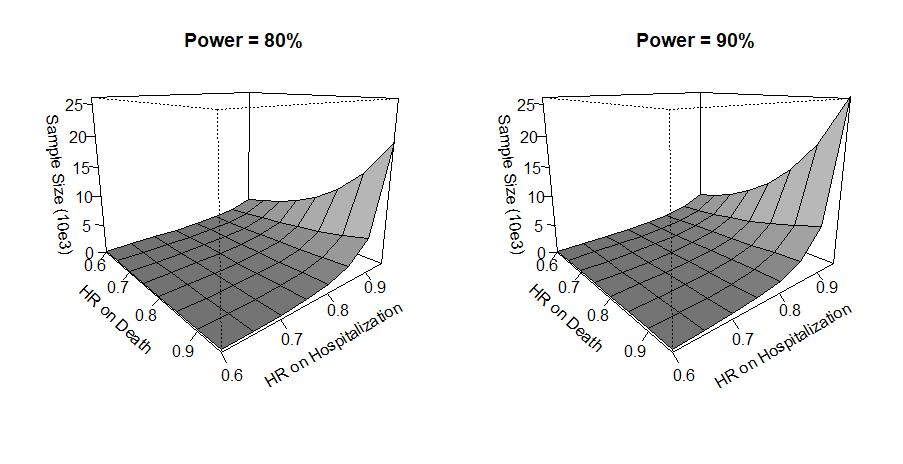
#> [1] 0.360812Sample Size: Example
- One scenario
- HRs on death & hospitalization: 0.9, 0.8
- Sample size needed for power 80%: \(n=1241\)
# set design parameters
tau_b <- 3
tau <- 4
lambda_L <- 0.001
# Step 2: use base() function to compute zeta2 and delta
set.seed(1234) # Monte-Carlo integration in base()
bparam <- base(lambda_D, lambda_H, kappa, tau_b, tau, lambda_L)
# Step 3: compute sample size under HRs 0.8 and 0.9
obj <- WRSS(xi = log(c(0.9, 0.8)), bparam = bparam, q =  0.5, alpha = 0.05,
          power = 0.8)
obj$n
#> [1] 1240.958
A Range of Effect Sizes
- Different HRs: \(\exp(\xi)\in [0.6, 0.95]^{\otimes 2}\)
Conclusion
Notes
- Event-specific win ratio
- Win/loss on which component (Yang et al., 2022; Yang & Troendle, 2020)
- More on sample size
- Calculatation based on win/loss proproportions (Yu & Ganju, 2022)
- Simplified/approximate approaches in various scenarios (Gasparyan et al., 2021; Seifu et al., 2022, etc.; Wang et al., 2023; Zhou et al., 2022)
Summary
- Win ratio test
- Standard: death > one nonfatal event
- Recurrent events: death > frequency > time to last/first event
WR::WRrec(ID, time, status, trt, strata)
- Sample size calculations
- Gumbel-Hougaard copula for death & nonfatal event \[\pr(D^\a>s, T_1^\a>t) = \exp\left(-\left[\{\exp(a\xi_D)\lambda_Ds\}^\kappa + \{\exp(a\xi_H)\lambda_Ht\}^\kappa \right]^{1/\kappa}\right)
\]
- Step 1: estimate \((\lambda_D,\lambda_H,\kappa)\)
WR::gumbel.est(id, time, status) - Step 2: calculate \(\zeta^2_0(\lambda_D,\lambda_H,\kappa,\tau_b,\tau,\lambda_L)\) and \(\delta(\lambda_D,\lambda_H,\kappa,\tau_b,\tau,\lambda_L)\)
WR::base() - Step 3: \(n=\frac{\zeta_0^2(\lambda_D,\lambda_H,\kappa,\tau_c,\tau,\lambda_L)(z_{1-\alpha/2} + z_\gamma)^2}{q(1-q)\delta(\lambda_D,\lambda_H,\kappa,\tau_c,\tau,\lambda_L)^\T\xi}\)
WR::WRSS()
- Step 1: estimate \((\lambda_D,\lambda_H,\kappa)\)
- Gumbel-Hougaard copula for death & nonfatal event \[\pr(D^\a>s, T_1^\a>t) = \exp\left(-\left[\{\exp(a\xi_D)\lambda_Ds\}^\kappa + \{\exp(a\xi_H)\lambda_Ht\}^\kappa \right]^{1/\kappa}\right)
\]