source("wrnet_functions.R")WRNet: Regularized win ratio regression through elastic net
Variable selection and risk prediction for hierarchical composite outcomes
WRNet is a machine-learning approach for regularized win ratio regression tailored to hierarchical composite endpoints. It optimizes feature selection and risk prediction through an elastic net-type penalty on regression coefficients (log-win ratios), making it suitable for high-dimensional data.
- Presentation (4/4/2025)
Basics
When comparing two subjects \(i\) vs \(j\) at time \(t\), a winner is defined as the subject with either:
- Longer overall survival, or
- Longer event-free survival, if both survive past \(t\).
In this way, death is prioritized over nonfatal events.
A basic win ratio model is expressed as: \[ \frac{P(\text{Subject $i$ wins by time $t$})}{P(\text{Subject $j$ wins by time $t$})} = \exp\{\beta^{\rm T}(z_i - z_j)\}. \] For high-dimensional covariates \(z\), the model is regularized using a combination of \(L_1\) (lasso) and \(L_2\) (ridge regression) penalties on \(\beta\).
A Step-by-Step Guide
Installation
Download and compile the R functions from the wrnet_functions.R script available at the GitHub repository.
Two packages used extensively in these functions are glmnet and tidyverse.
library(glmnet) # for elastic net
library(tidyverse) # for data manipulation/visualization
Data preparation
Consider a German breast cancer study with 686 subjects and 9 covariates.
# Load package containing data
library(WR)
# Load data
data("gbc")
df <- gbc # n = 686 subjects, p = 9 covariates
df # status = 0 (censored), 1 (death), 2 (recurrence)
#>   id      time status hormone age menopause size grade ...
#>1   1 43.836066      2       1  38         1   18     3
#>2   1 74.819672      0       1  38         1   18     3
#>3   2 46.557377      2       1  52         1   20     1
#>4   2 65.770492      0       1  52         1   20     1
#>5   3 41.934426      2       1  47         1   30     2
#>...
Split data into training versus test set:
# Data partitioning ------------------------------------
set.seed(123)
obj_split <- df |> wr_split() # default: 80% training, 20% test
# Take training and test set
df_train <- obj_split$df_train
df_test <- obj_split$df_test
Tuning-parameter selection
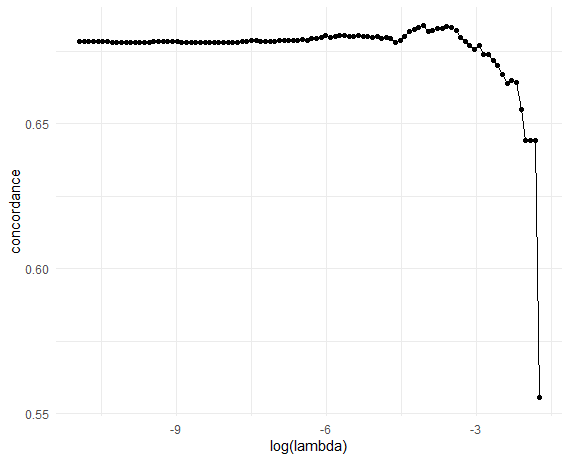
Perform 10-fold (default) cross-validationon the training set:
# 10-fold CV -------------------------------------------
set.seed(1234)
obj_cv <- cv_wrnet(df_train$id, df_train$time, df_train$status,
                    df_train |> select(-c(id, time, status)))
# Plot CV results (C-index vs log-lambda)
obj_cv |>
   ggplot(
    aes(x =  log(lambda), y = concordance)
   ) +
   geom_point() +
   geom_line() +
   theme_minimal()
Retrieve the optimal \(\lambda\):
# Optimal lambda
lambda_opt <- obj_cv$lambda[which.max(obj_cv$concordance)]
lambda_opt
#> [1] 0.0171976
Final model and evaluation
Finalize model at optimal tuning parameter \(\lambda_{\rm opt}\):
# Final model ------------------------------------------
final_fit <- wrnet(df_train$id, df_train$time, df_train$status,
              df_train |> select(-c(id, time, status)),
              lambda = lambda_opt)
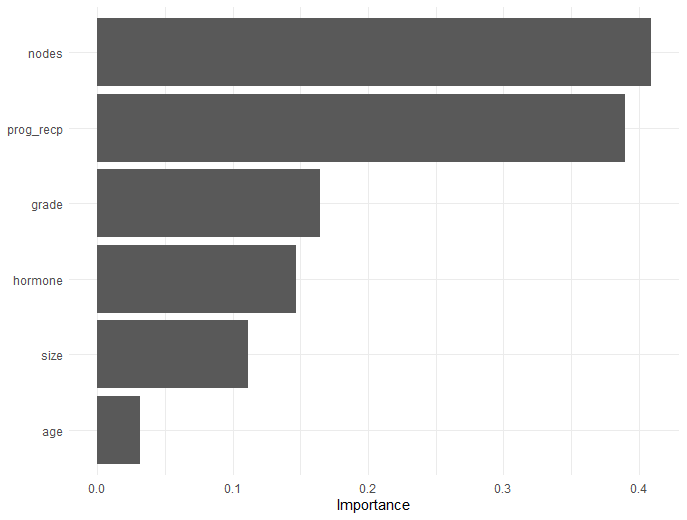
# Estimated coefficients
final_fit$beta
#> 8 x 1 sparse Matrix of class "dgCMatrix"
#>                      s0
#> hormone     0.306026364
#> age         0.003111462
#> menopause   .
#> size       -0.007720497
#> grade      -0.285511701
#> nodes      -0.082227827
#> prog_recp   0.001861367
#> estrg_recp  .
# Variable importance plot
final_fit |>
   vi_wrnet() |>
   vip()
Evaluate model performance through C-index:
# Test model performance -------------------------------
test_result <- final_fit |> test_wrnet(df_test)
# Overall and event-specific C-indices
test_result$concordance
#> # A tibble: 3 × 2
#>   component concordance
#>   <chr>           <dbl>
#> 1 death           0.724
#> 2 nonfatal        0.607
#> 3 overall         0.664
Note
Both cv_wrnet() and wrnet() functions accept additional arguments and pass them to the underlying glmnet::glmnet(). For example, setting alpha = 0.5 applies an equal mix of lasso and ridge penalties (default: alpha = 1 for lasso).