# Load library
library(tidyverse)How to do efficient simulations using Tidyverse
General steps
- Generate multiple datasets: Simulate \(N\) datasets based on a defined data-generating process.
- Apply a statistical method: For each dataset, apply the same statistical method (e.g., linear regression, hypothesis testing).
- Summarize the results: Aggregate and summarize performance metrics (e.g., bias, MSE, coverage).
Example: linear regression
Consider a simulation study for linear regression.
Define the data-generating process
Simulate a dataset for linear regression:
generate_data <- function(n = 100, beta0 = 1, beta1 = 2, sigma = 1) {
  tibble(
    x = rnorm(n),
    y = beta0 + beta1 * x + rnorm(n, sd = sigma)
  )
}
Define the statistical method
Fit a linear model and extract the coefficient estimates:
fit_model <- function(data) {
  model <- lm(y ~ x, data = data)
  tibble(
    beta0_hat = coef(model)[1],
    beta1_hat = coef(model)[2]
  )
}
Perform simulation
Generate \(N = 1000\) datasets, each with an id (sim_id) and stored in a list-valued column data.
set.seed(123)

# Number of simulations
N <- 1000

# Simulate data
simulated_data <- tibble(
  sim_id = 1:N
) %>%
  mutate(
    data = map(sim_id, ~ generate_data(n = 100, beta0 = 1, beta1 = 2, sigma = 1)) # Generate datasets
  )

 ## Take a look
simulated_data
# A tibble: 1,000 × 2
sim_id data
<int> <list>
1 1 <tibble [100 × 2]>
2 2 <tibble [100 × 2]>
3 3 <tibble [100 × 2]>
4 4 <tibble [100 × 2]>
5 5 <tibble [100 × 2]>
6 6 <tibble [100 × 2]>
7 7 <tibble [100 × 2]>
8 8 <tibble [100 × 2]>
9 9 <tibble [100 × 2]>
10 10 <tibble [100 × 2]>
# ℹ 990 more rowsUse purrr::map() to fit a linear model to each entry of data and store the results in a list-valued column results. Then unnest to combine all results into a single table.
# Fit model to each simulated dataset
simulation_results <- simulated_data %>%
  mutate(
   results = map(data, fit_model) # Apply the model
  ) %>%
  unnest(results) # Combine all results into a single table

## Take a look
simulation_results
# A tibble: 1,000 × 4
sim_id data beta0_hat beta1_hat
<int> <list> <dbl> <dbl>
1 1 <tibble [100 × 2]> 0.897 1.95
2 2 <tibble [100 × 2]> 0.970 1.95
3 3 <tibble [100 × 2]> 0.937 2.20
4 4 <tibble [100 × 2]> 1.11 2.00
5 5 <tibble [100 × 2]> 0.983 1.98
6 6 <tibble [100 × 2]> 0.979 2.02
7 7 <tibble [100 × 2]> 0.940 1.99
8 8 <tibble [100 × 2]> 1.04 1.96
9 9 <tibble [100 × 2]> 1.03 1.98
10 10 <tibble [100 × 2]> 1.08 1.94
# ℹ 990 more rows# Summarize the results
summary_stats <- simulation_results %>%
summarize(
beta0_mean = mean(beta0_hat),
beta1_mean = mean(beta1_hat),
beta0_bias = mean(beta0_hat - 1),
beta1_bias = mean(beta1_hat - 2),
beta0_sd = sd(beta0_hat),
beta1_sd = sd(beta1_hat)
)
summary_stats# A tibble: 1 × 6
beta0_mean beta1_mean beta0_bias beta1_bias beta0_sd beta1_sd
<dbl> <dbl> <dbl> <dbl> <dbl> <dbl>
1 1.00 2.00 0.00336 0.00357 0.102 0.103Visualize the results (optional)
# Histogram of beta1 estimates
ggplot(simulation_results, aes(x = beta1_hat)) +
  geom_histogram(bins = 30, fill = "skyblue", color = "black") +
  geom_vline(xintercept = 2, linetype = "dashed", color = "red") +
  labs(
    title = "Distribution of Beta1 Estimates",
    x = "Beta1 Estimates",
    y = "Frequency"
  ) +
  theme_minimal()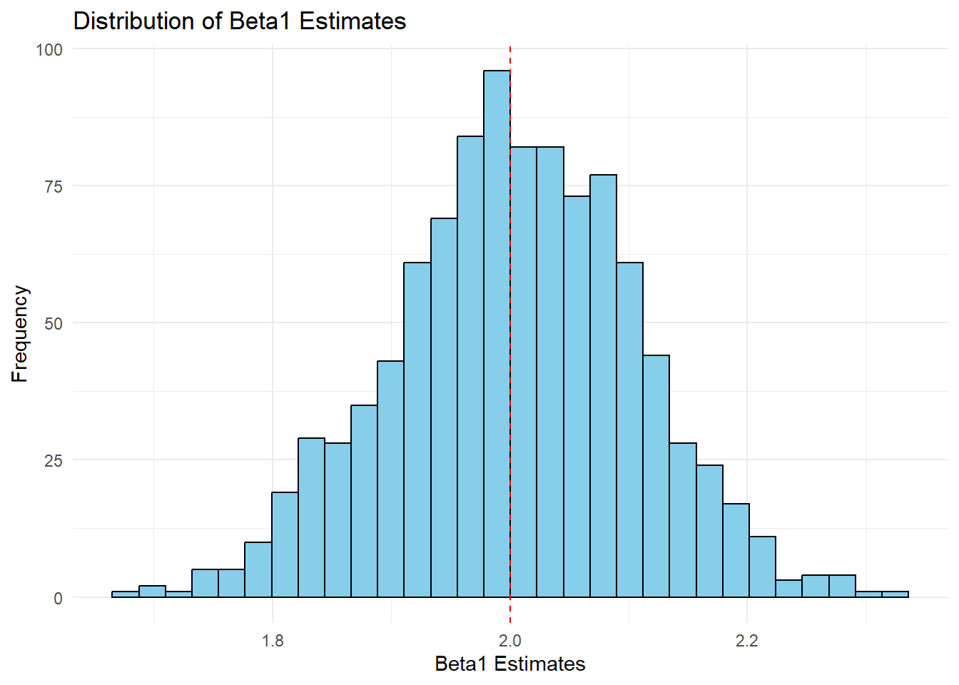
Key features of workflow
- Reproducibility:
- Use
set.seed()for consistent results.
- Use
- Scalability:
- Adjust
Nto increase or decrease the number of datasets.
- Adjust
- Summarization:
map()andunnest()make it easy to handle multiple datasets and their outputs.
- Customization:
- Replace the data-generating process or statistical method to fit your needs.