# Load required packages
library(tidyverse)
library(irr)  # For ICC calculation
library(knitr)  # For table formatting

# Simulating data
set.seed(123)
data <- tibble(
  Biomarker = rep(c("A", "B", "C"), each = 50),
  Method1 = rnorm(150, mean = 10, sd = 2),
  Method2 = rnorm(150, mean = 10, sd = 2)
)
head(data)
#> # A tibble: 6 × 3
#>   Biomarker Method1 Method2
#>   <chr>       <dbl>   <dbl>
#> 1 A            8.88   11.6
#> 2 A            9.54   11.5
#> 3 A           13.1    10.7
#> 4 A           10.1     7.98
#> 5 A           10.3     9.76
#> 6 A 13.4 9.44How to create Bland-Altman analysis for multiple biomarkers
Use group_by() for agreement statistics and facet_wrap() for plots
Bland-Altman analysis is a popular method to assess agreement between two measurement methods. When dealing with multiple biomarkers, it’s essential to analyze each biomarker separately while ensuring a consistent set of statistics and visualizations are applied. In this post, I’ll show you how to:
- Use
dplyrto calculate the Intraclass Correlation Coefficient (ICC) or Concordance Correlation Coefficient (CCC) with their 95% confidence intervals. - Create faceted Bland-Altman plots with key statistics (bias, limits of agreement) labeled on each panel.
Let’s dive in using a simulated dataset for clarity.
Simulated data example
Calculate ICC for each biomarker
Using dplyr’s group_by() function, we can calculate the ICC for each biomarker and extract 95% confidence intervals.
# Calculate ICC for each biomarker
icc_results <- data %>%
  group_by(Biomarker) %>%
  summarize(
    ICC = round(icc(cbind(Method1, Method2), model = "twoway", type = "agreement")$value, 3),
    LowerCI = round(icc(cbind(Method1, Method2), model = "twoway", type = "agreement")$lbound, 3),
    UpperCI = round(icc(cbind(Method1, Method2), model = "twoway", type = "agreement")$ubound, 3)
  )

# Display ICC results as a formatted table
kable(icc_results, align = "c")| Biomarker | ICC | LowerCI | UpperCI |
|---|---|---|---|
| A | -0.125 | -0.396 | 0.162 |
| B | -0.129 | -0.395 | 0.154 |
| C | -0.168 | -0.400 | 0.097 |
Create Bland-Altman plots
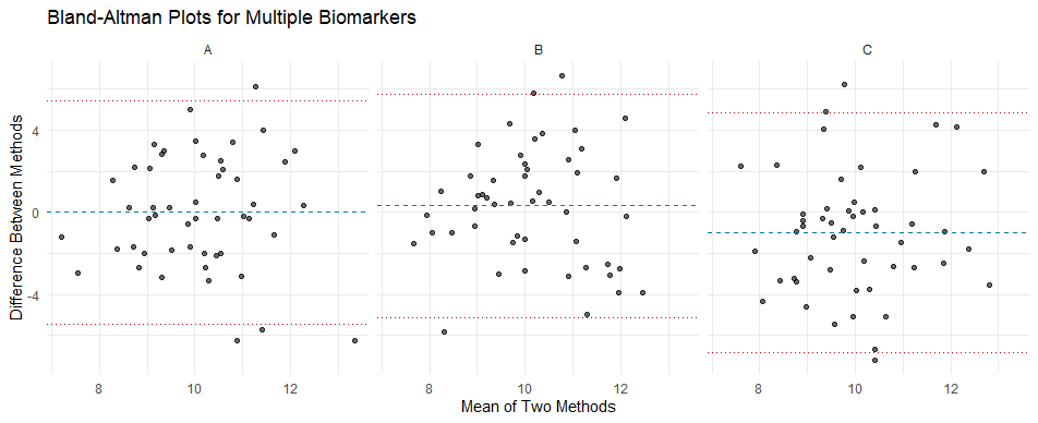
We’ll calculate the mean and difference of the two methods for each biomarker, then use facet_wrap() to create individual plots for each biomarker. Key statistics like bias and limits of agreement (LoA) will be annotated on each panel.
# Add Bland-Altman calculations to the data
data <- data %>%
  mutate(
    # Calculate the mean of the two methods for each observation
    Mean = (Method1 + Method2) / 2,
    # Calculate the difference between the two methods for each observation
    Difference = Method1 - Method2
  )

# Bland-Altman plot function
plot_bland_altman <- function(data) {
  data %>%
    group_by(Biomarker) %>% # Group data by each biomarker
    summarize(
      # Calculate the bias (mean difference) for each biomarker
      Bias = mean(Difference),
      # Calculate the lower limit of agreement (LoA)
      LoA_Lower = Bias - 1.96 * sd(Difference),
      # Calculate the upper limit of agreement (LoA)
      LoA_Upper = Bias + 1.96 * sd(Difference)
    ) %>%
    # Merge the summary statistics (Bias, LoA) back into the original data for plotting
    left_join(data, by = "Biomarker") %>%
    ggplot(aes(x = Mean, y = Difference)) + # Plot mean (x) vs. difference (y)
    geom_point(alpha = 0.6) + # Add scatter points with slight transparency
    geom_hline(aes(yintercept = Bias), color = "#0479A8", linetype = "dashed") +
    # Add a horizontal dashed line for the bias (mean difference)
    geom_hline(aes(yintercept = LoA_Lower), color = "#C5050C", linetype = "dotted") +
    # Add a dotted horizontal line for the lower limit of agreement
    geom_hline(aes(yintercept = LoA_Upper), color = "#C5050C", linetype = "dotted") +
    # Add a dotted horizontal line for the upper limit of agreement
    facet_wrap(~ Biomarker) + # Create separate panels for each biomarker
    labs(
      title = "Bland-Altman Plots for Multiple Biomarkers", # Set plot title
      x = "Mean of Two Methods", # Label for the x-axis
      y = "Difference Between Methods" # Label for the y-axis
    ) +
    theme_minimal() # Use a clean, minimal theme for the plot
}

# Create Bland-Altman plots
plot_bland_altman(data) # Call the function to generate and display the plots
Summary
With just a few lines of code, we’ve:
- Calculated the ICC (or CCC) for each marker, complete with confidence intervals.
- Created a clear and concise Bland-Altman plot using
facet_wrap()for each marker.
These steps provide a straightforward way to analyze agreement for multiple biomarkers simultaneously, saving a lot of effort.