WRNet: Regularized win ratio regression
Variable selection and risk prediction with hierarchical composite outcomes
Department of Biostatistics & Medical Informatics
University of Wisconsin-Madison
\[ \newcommand{\wh}{\widehat} \newcommand{\wt}{\widetilde} \def\bs{\boldsymbol} \newcommand{\red}{} \newcommand{\indep}{\perp \!\!\! \perp} \def\T{{ \mathrm{\scriptscriptstyle T} }} \def\pr{{\rm pr}} \def\d{{\rm d}} \def\W{{\mathcal W}} \def\H{{\mathcal H}} \def\I{{\mathcal I}} \def\C{{\mathcal C}} \def\S{{\mathcal S}} \def\Sk{{\mathcal S}^{(k)}} \def\Skm{{\mathcal S}^{(-k)}} \def\v{\varepsilon} \def\bSig\mathbf{\Sigma} \def\Un{\sum_{i=1}^{n-1}\sum_{j=i+1}^n} \]
Outline
- Introduction
- Methods
- Standard win ratio regression
- Regularization and computation
WRNetworkflow
- Simulation studies
- HF-ACTION application
Introduction
Hierarchical Composite Endpoints
- Composite outcomes
- Components: Death, hospitalization, other events
- Standard approach: Time to first event (e.g., Cox model)
- Win ratio (WR) (Pocock et al., 2012)
- Pairwise comparisons: Treatment vs control (Buyse, 2010)
- Each pair: Death > hospitalization (> other events)
- Effect size \[ \text{WR} = \frac{\text{Number of wins}}{\text{Number of losses}} \]
Data and Notation
- Outcomes data (subject \(i\))
- \(D_i\): time to death
- \(T_i\): time to first nonfatal event
- \(\bs Y_i(t) =(D_i\wedge t, T_i\wedge t)\): cumulative data at \(t\)
- \(x\wedge y = \min(x, y)\)
- Win indicator \[\begin{align*}\label{eq:win2tier} \W(\bs Y_i, \bs Y_j)(t) = \underbrace{I(D_j< D_i\wedge t)}_{\mbox{Win on survival}} + \underbrace{I(D_i\wedge D_j >t,\; T_j< T_i\wedge t)}_ {\mbox{Tie on survival, win on nonfatal event}} \end{align*}\]
Win Ratio Regression
- Semiparametric regression \[\begin{equation}\label{eq:pw}
\frac{\pr\{\W(\bs Y_i, \bs Y_j)(t) = 1\mid z_i, z_j\}}{\pr\{\W(\bs Y_j, \bs Y_i)(t) = 1\mid z_j, z_i\}} = \exp\left\{\beta^\T(z_i - z_j)\right\}
\end{equation}\]
- \(z\): \(p\)-dimensional covariates
- Proportional win-fractions (PW) model
- Equivalent to Cox PH model in univariate case (Oakes, 2016)—WR = 1/HR
- \(\exp(\beta)\): win ratios associated with unit increases in \(z\)
- Limitation: \(p<< n\)
Goals
- Objectives:
- Automate variable selection in WR regression
- Enhance prediction accuracy and model parsimony
- Automate variable selection in WR regression
- Approach:
- Apply elastic net regularization to PW model
- Mixture of \(L_1\) (lasso) and \(L_2\) (ridge) penalties
- Mixture of \(L_1\) (lasso) and \(L_2\) (ridge) penalties
- Implemented in
wrnetR package
- Apply elastic net regularization to PW model
Methods
Standard Model-Fitting
- Observed data
- \(\bs Y_i(X_i)\): outcomes data up to \(X_i = D_i \wedge C_i\) (\(C_i\): censoring time)
- Estimating equation (Mao & Wang, 2021) \[\begin{equation}
U_n(\beta) = |\mathcal R|^{-1} \sum_{(i, j)\in \mathcal R}
z_{ij} \left\{ \delta_{ij} - \frac{\exp(\beta^\top z_{ij})}{1 + \exp(\beta^\top z_{ij})} \right\}
\end{equation}\]
- \(z_{ij} = z_i - z_j\): covariate difference
- \(\delta_{ij} = \mathcal{W}(\bs Y_i, \bs Y_j)(X_i \wedge X_j)\): observed win indicator
- \(\mathcal{R}=\{(i, j): \delta_{ij} + \delta_{ji} > 0\}\): set of comparable pairs
- \(z_{ij} = z_i - z_j\): covariate difference
Estimation
- Estimator: solving \[
U_n(\hat\beta) \;\;= 0
\]
- Standard Newton–Raphson algorithm
- Connection with logistic regression
- \(U_n(\hat\beta)\) equivalent to logistic score function (no intercept)
- Each comparable \((i, j)\) pair as an observation
- \(\delta_{ij}\): binary response
- \(z_{ij}\): covariates
Regularized PW model
- Objective function (Zou & Hastie, 2005): \[\begin{align}\label{eq:obj_fun}
l_n(\beta;\lambda) &= - |\mathcal R|^{-1}\sum_{(i, j)\in\mathcal R}\left[\delta_{ij}\beta^\T z_{ij} - \log\{1+\exp(\beta^\T z_{ij})\}\right]\notag\\
&\hspace{3em}+\lambda\left\{(1-\alpha)||\beta||_2^2/2+\alpha||\beta||_1\right\}
\end{align}\]
- Pathwise solution \(\hat\beta(\lambda) = \arg\min_\beta l_n(\beta;\lambda)\)
- Numerically equivalent to regularized logistic regression
- Tuning parameter \(\lambda\geq 0\)—determined by cross-validation (CV)
- \(\partial l_n(\beta; 0)/\partial\beta = U_n(\beta)\)
- Mixing parameter \(\alpha \in (0, 1)\)
- \(\alpha > 0\) \(\longrightarrow\) some components of \(\hat\beta(\lambda)=0\) (performs variable selection)
- Pathwise solution \(\hat\beta(\lambda) = \arg\min_\beta l_n(\beta;\lambda)\)
Pathwise Solution
Pathwise algorithm (Friedman et al., 2010)
- Efficient computation of \(\hat\beta(\lambda)\) for all \(\lambda\)
x: covariate matrix containing \(z_{ij}\) ,y: response vector \(\delta_{ij}\)intercept = FALSEremoves interceptlambda: user-specified \(\lambda\) vector
Cross Validation
- CV routine for logistic regression
cv.glmnet()- Partition pairs into \(k\) folds—train and validate
- Built-in
cv.glmnet() - Not appropriate
- Overlap between analysis and validation sets
- Inflation of sample size
- Subject-based CV
- Partition subjects into \(k\) folds \(\mathcal{S}^{(k)}\)
- Train on \(\mathcal{S}^{(-k)}\): \(\wh\beta^{(-k)}(\lambda)\) \(\longrightarrow\) validate on \(\mathcal{S}^{(k)}\)
- Identify optimal \(\lambda\) maximizing average concordance index
Win/Risk Score
- Motivation
- Model-predicted win probability given comparability \[\mu(z_i, z_j;\beta)=\frac{\exp\{\beta^\T(z_i-z_j)\}}{1 + \exp\{\beta^\T(z_i-z_j)\}}\]
- \(\beta^\T z\) measures tendency to win \[\begin{align*} \mu(z_i, z_j;\beta) > 0.5 &\Leftrightarrow \beta^\T z_i > \beta^\T z_j;\\ \mu(z_i, z_j;\beta) = 0.5 &\Leftrightarrow \beta^\T z_i = \beta^\T z_j;\\ \mu(z_i, z_j;\beta) < 0.5 &\Leftrightarrow \beta^\T z_i < \beta^\T z_j. \end{align*}\]
- \(-\beta^\T z\): risk score
Generalized Concordance Index
- Validation/test set \(\mathcal S^*\)
- Pairwise indices \[ \mathcal R^* = \{(i,j): \delta_{ij}+\delta_{ji}\neq 0; i<j; i,j\in\S^*\} \]
- Concordance (Cheung et al., 2019; Harrell et al., 1982; Uno et al., 2011)
- Proportion of correct ranking of pairs \[\begin{equation}\label{eq:c_index} \mathcal C(\S^*;\beta) = |\mathcal R^*|^{-1}\sum_{(i, j)\in\mathcal R^*} \bigl[\underbrace{I\{(2\delta_{ij} -1)(\beta^\T z_i - \beta^\T z_j)>0\}}_{\text{Concordant pair}}+2^{-1} \underbrace{I(\beta^\T z_i = \beta^\T z_j)}_{\text{Tied score}}\bigr] \end{equation}\]
Validation and Testing
- Model tuning
- \(k\)th-fold CV concordance: \(C^{(k)}(\lambda) = \mathcal C\left(\Sk;\wh\beta^{(-k)}(\lambda)\right)\)
- Optimal \(\lambda_{\rm opt} = \arg\max_\lambda K^{-1}\sum_{k=1}^K\C^{(k)}(\lambda)\)
- Final model: \(\wh\beta(\lambda_{\rm opt})\)
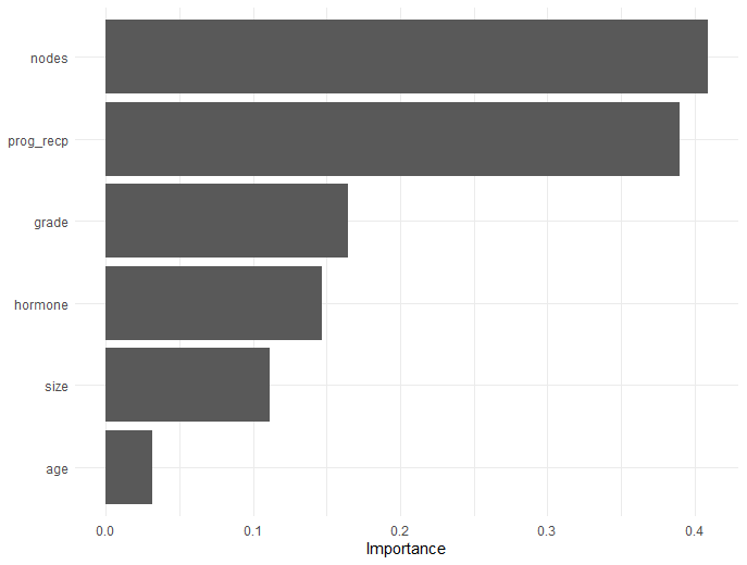
- Variable importance
- Component-wise \(|\beta|/\text{sd}(z)\)
- Test C-index
- \(\mathcal C(\S^*;\wh\beta(\lambda_{\rm opt}))\) for test set \(\S^*\)
Workflow - Input Data
Data format
- Long format with columns:
id,time,status, and covariates
# Load package containing data library(WR) df <- gbc # n = 686 subjects, p = 9 covariates df # status = 0 (censored), 1 (death), 2 (recurrence) #> id time status hormone age menopause size grade ... #>1 1 43.836066 2 1 38 1 18 3 #>2 1 74.819672 0 1 38 1 18 3 #>3 2 46.557377 2 1 52 1 20 1 #>4 2 65.770492 0 1 52 1 20 1 #>5 3 41.934426 2 1 47 1 30 2 #>...- Long format with columns:
Workflow - Data Partitioning
- Splitting data
wr_split()function
Workflow - Cross-Validation (I)
- \(k\)-fold CV
cv_wrnet(id, time, status, Z, k = 10, ...)
# 10-fold CV -------------------------------------------
set.seed(1234)
obj_cv <- cv_wrnet(df_train$id, df_train$time, df_train$status,
df_train |> select(-c(id, time, status)))
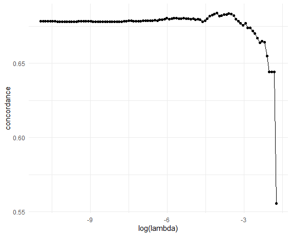
# Plot CV results (C-index vs log-lambda)
obj_cv |>
ggplot(aes(x = log(lambda), y = concordance)) +
geom_point() + geom_line() + theme_minimal()
# Optimal lambda
lambda_opt <- obj_cv$lambda[which.max(obj_cv$concordance)]
lambda_opt
#> [1] 0.0171976Workflow - Cross-Validation (II)
- Validation C-index
Workflow - Final Model
Fit final model
wrnet(id, time, status, Z, lambda = lambda_opt, ...)
# Final model ------------------------------------------
final_fit <- wrnet(df_train$id, df_train$time, df_train$status,
          df_train |> select(-c(id, time, status)), lambda = lambda_opt)
final_fit$beta # Estimated coefficients
#>                      s0
#> hormone     0.306026364
#> age         0.003111462
#> menopause   .
#> size       -0.007720497
#> grade      -0.285511701
#> nodes      -0.082227827
#> prog_recp   0.001861367
#> estrg_recp  .
Workflow - Variable Importance
- Variable importance
Workflow - Test Performance
- Overall and component-wise C-index
test_wrnet(final_fit, df_test)
Simulations
Setup
- Covariates: \(z = (z_{\cdot 1}, z_{\cdot 2}, \ldots, z_{\cdot p})^\T\)
- \(z_{\cdot k} \sim N(0,1)\)—AR(1) with \(\rho = 0.1\)
- Outcome model: \[
\pr(D > s, T > t\mid z) = \exp\left(-\left[\{\exp(-\beta_D^\T z)\lambda_Ds\}^\kappa + \{\exp(-\beta_H^\T z)\lambda_Ht\}^\kappa\right]^{1/\kappa}\right)
\]
- \(\lambda_D = 0.1\), \(\lambda_H = 1\), \(\kappa = 1.25\)
- Censoring: \(\mbox{Un}[0.2, 4]\wedge\mbox{Expn}(\lambda_C)\)
- \(\lambda_C = 0.02\)
Two Effect Patterns
- Scenarios
- Same effect pattern on components \[ \beta_D=\beta_H=(\underbrace{0.5,\ldots, 0.5}_{10}, \underbrace{0,\ldots, 0}_{p - 10}). \]
- Different effect patterns on components \[\begin{align*} \beta_D&=(\underbrace{0.75,\ldots, 0.75}_{5}, \underbrace{0,\ldots, 0}_{p - 5});\\ \beta_H&=(\underbrace{0,\ldots, 0}_{5}, \underbrace{0.75,\ldots, 0.75}_{5}, \underbrace{0,\ldots, 0}_{p - 10}) \end{align*}\]
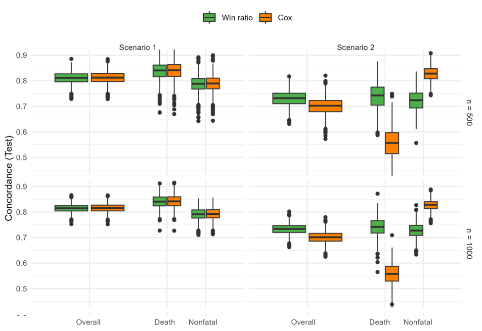
Predictive Accuracy - C-index
- Regularized WR vs regularized Cox on first event
- 80% training + 20% testing
Variable Selection - Sensitivity
- S2: \(z_{\cdot 1}\)–\(z_{\cdot 5}\) \(\longrightarrow\) mortality
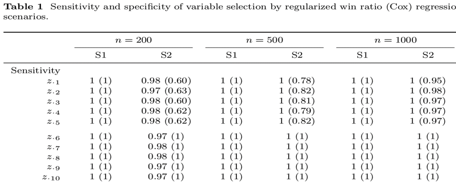
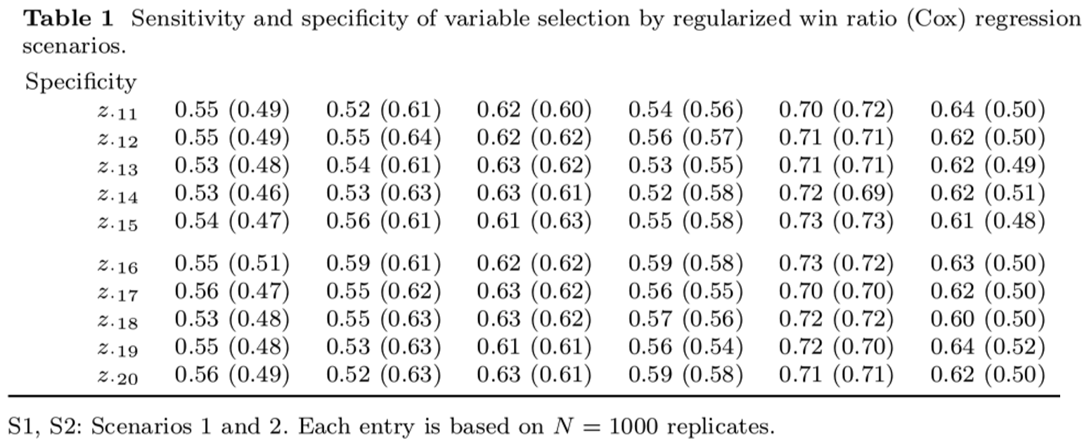
Variable Selection - Specifity
- \(z_{\cdot 11}\)–\(z_{\cdot 20}\) \(\longrightarrow\) no effect
HF-ACTION Application
Study Information
- HF-ACTION (O’Connor et al., 2009)
- Population: 2,331 HFrEF patients across North America and France
- Objective: Evaluate the effect of exercise training on composite of death and hospitalization
- Subgroup of high-risk patients
- \(n=426\) high-risk patients (CPX duration \(\leq 9\) min)
- Outcomes: death > hospitalization
- \(p=153\) baseline features
- Train-test split: 80%/20%
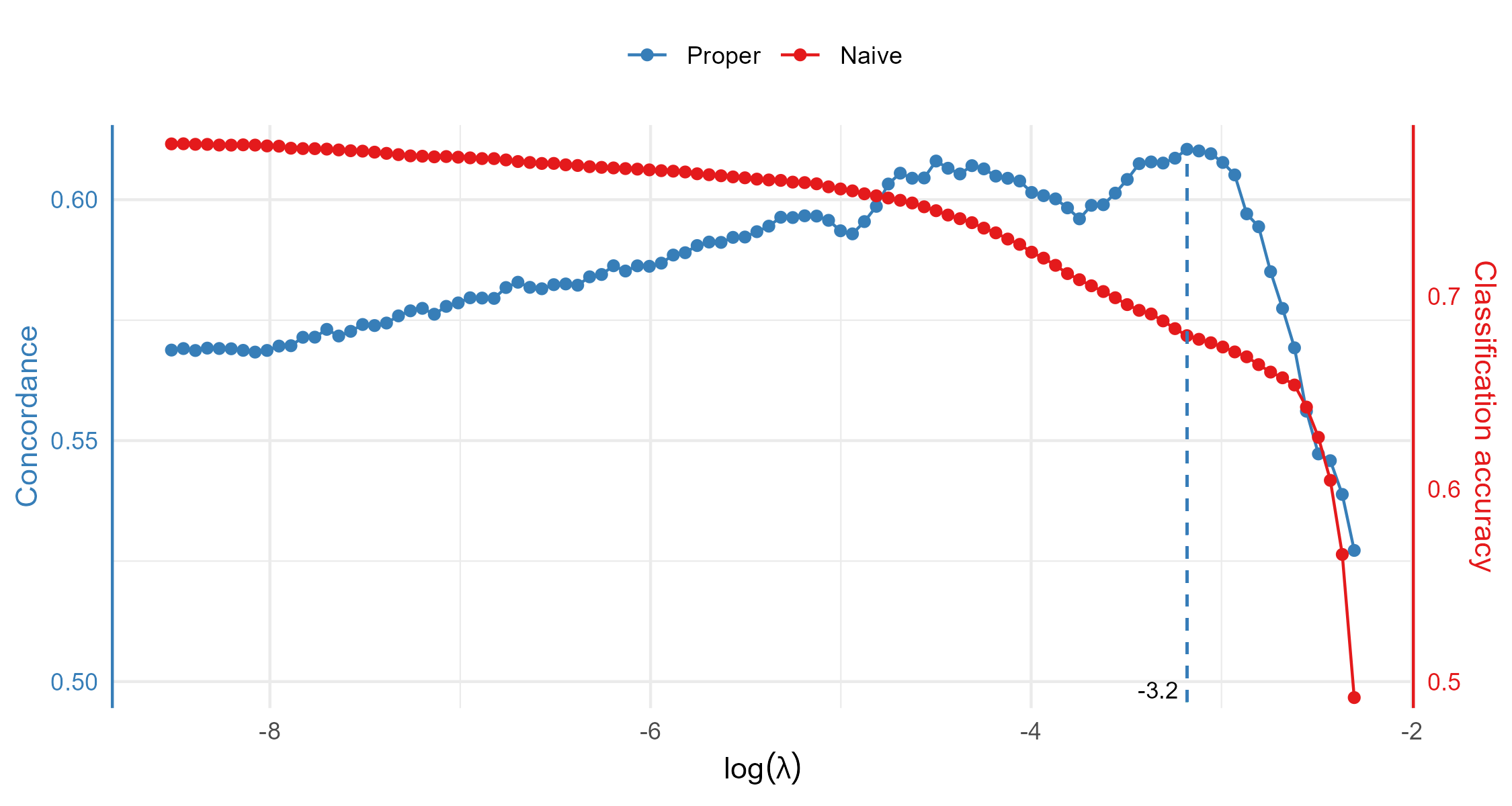
Cross-Validation
- Naive pairwise logistic CV on pairs leads to overfitting
Test Performance - Risk Scores
- WRNet vs regularized Cox
- WRNet better stratifies high-risk patients, especially on mortality

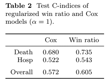
Test Performance - C-Index
- WRNet vs regularized Cox
- WRNet outperforms Cox on overall and event-specific C-indices
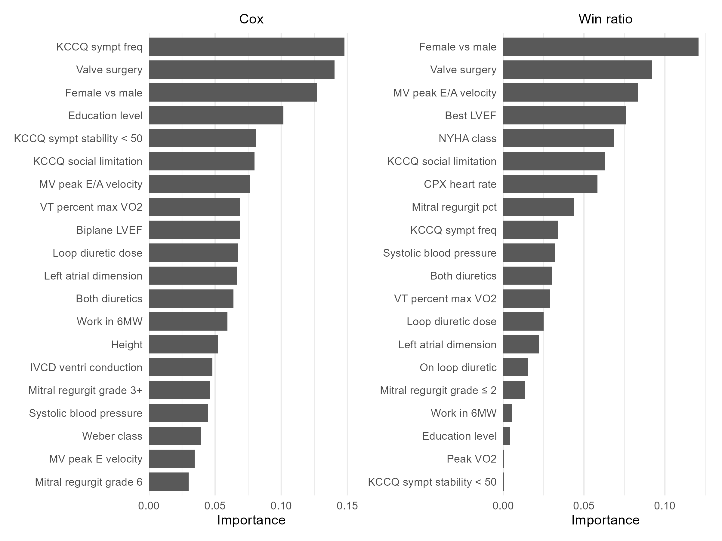
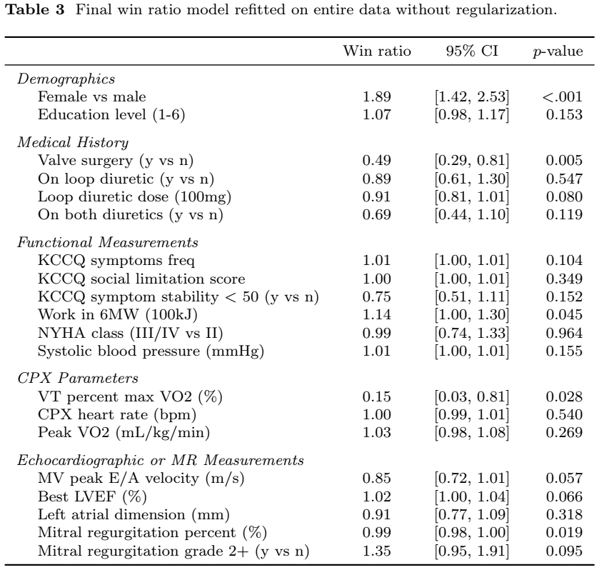
Variable Importance
- WRNet selects 20 interpretable variables
![]()
Final WR Model
Summary and Discussion
Summary
- Methodology
- Developed elastic net-regularized WR regression
- Better aligns with clinical priorities than Cox
- Accurate feature selection and prediction
- Tools
wrnet: https://lmaowisc.github.io/wrnet/- Efficient implementation with
glmnet()backend - Supports CV, test evaluation, and variable importance
Future Topics
- Explore \(\alpha \in (0,1)\) settings
- Extend to time-varying effects and nonlinearities
- Decision trees