WinKM: Approximating win-loss probabilities
Using overall and event-free survival functions
Department of Biostatistics & Medical Informatics
University of Wisconsin-Madison
Visit https://lmaowisc.github.io/winKM
\[ \newcommand{\wh}{\widehat} \newcommand{\wt}{\widetilde} \def\bs{\boldsymbol} \newcommand{\red}{} \newcommand{\indep}{\perp \!\!\! \perp} \]
Outline
- Introduction
- Methods
- Win-loss estimands
- Approximating formula
WinKMworkflow
- Case studies
- A colon cancer trial
- HF-ACTION trial
- Conclusion
Introduction
- Win-loss statistics
- Generalized pairwise comparisons (GPC) (Buyse et al., 2025)
- Prioritization: death > nonfatal event (hospitalization/disease progression)
- Proportions of wins vs losses
- Win ratio (Pocock et al., 2012), win odds (Brunner et al., 2021), net benefit (Buyse, 2010)
- Meta analysis?
- Literature-wide evidence synthesis
- Earlier studies not reporting win-loss measures
- Patient-level data unavailable
Methods
Notation
- Outcome data
- \(D_a\): Overall survival (OS) time
- \(T_a\): Nonfatal event time
- \(T_a^* = D_a\wedge T_a\): Event-free survival (EFS) time
- \(a = 1\): treatment; 0: control
- Summary functions
- Joint survival: \(H_a(t, s)=\mathrm{pr}(T_a>t, D_a> s)\) - likely unavailable
- OS: \(S_a(t) =\mathrm{pr}(D_a > t)\) - available through Kaplan-Meier (KM) curve
- EFS: \(S_a^*(t) =\mathrm{pr}(T_a^* > t)\) - available through KM curve
Win-Loss Estimands
- Win-loss probabilities (Oakes, 2016)\[\begin{align}
w_{a, 1-a}(\tau) &= \mathrm{pr}(\mbox{Group $a$ wins by time $\tau$})\notag\\
&=\mathrm{pr}\underbrace{(D_{1-a}<D_a\wedge \tau)}_{\mbox{Win on OS}} +
\mathrm{pr}\underbrace{(D_1\wedge D_0 >\tau, T_{1-a}<T_a\wedge \tau)}_{\mbox{Tie on OS,
win on nonfatal}}\notag\\
&= \int_0^\tau \color{blue}{S_a(t-)\mathrm{d} F_{1-a}(t)}
\quad\quad\quad\quad \big(F_a(t) = 1 - S_a(t)\big)\\
&\hspace{1em}+\color{blue}{S_1(\tau)S_0(\tau)} \int_0^\tau \color{red}{\mathrm{pr}(T_a >t\mid D_a>\tau) \mathrm{pr}(t\leq T_{1-a} <t +\mathrm{d} t\mid D_{1-a}>\tau)}
\end{align}\]
- Win ratio: \(w_{1,0}(\tau)/w_{0,1}(\tau)\)
- Win odds: \(w_{1,0}(\tau)/w_{0,1}(\tau)\)
- Net benefit: \(w_{1,0}(\tau) - w_{0,1}(\tau)\)
Survival-Conditional Event Rate
- Second-term unknown \[\begin{align}
&\int_0^\tau \color{red}{\mathrm{pr}(T_a >t\mid D_a>\tau) \mathrm{pr}(t\leq T_{1-a} <t +\mathrm{d} t\mid D_{1-a}>\tau)}\\
=& -\int_0^\tau \color{red}{H_a(t\mid \tau) H_{1-a}(\mathrm{d} t\mid \tau)}\\
=&\,\color{red}{\mathrm{pr}(T_{1-a}<T_a\wedge \tau\mid D_1 > \tau, D_0 >\tau)}
\end{align}\]
- \(H_a(t\mid \tau)=\mathrm{pr}(T_a>t\mid D_a>\tau)\): event-free probabilities in \(\tau\)-survivors
- Association between death and nonfatal event
- Approximate it using \(S_a(t), S^*_a(t)\), and component-specific event counts
Approxmation - Idea
- Start with \(t\)-survivors \[\begin{align}
\mathrm{d}\Lambda_a(t\mid\tau) &:= \mathrm{pr}(t\le T_a < t + \mathrm{d} t\mid T_a\geq t, D_a>\color{red}{\tau})\\
&\leq \mathrm{pr}(t\le T_a < t + \mathrm{d} t\mid T_a\geq t, D_a\geq \color{red}{t})\\
&\approx \frac{N_a^{\rm E}}{N_a^*}\mathrm{d}\hat\Lambda_a^*(u)
\end{align}\]
- Notation
- \(N_a^{\rm E}\): number of nonfatal events
- \(N_a^*\): number of composite (EFS) endpoints
- \(\hat\Lambda_a^*(t)=-\log \hat S_a^*(t)\): cumulative hazard of EFS
- Inequality when cross ratio \(\kappa(t, s)\geq 1\) (positive association)
- Make up for bias by approximating \(\kappa(t, s)\)
- Notation
Cross Ratio
- Local dependence (Oakes, 1982, 1986) \[\begin{align*}\label{eq:cr:def}
\kappa_a(t, s) &=\frac{\mathrm{pr}(t\leq T_a< t +\mathrm{d} t\mid T_a\geq t, D_a = s )}
{\mathrm{pr}(t\leq T_a< t +\mathrm{d} t\mid T_a\geq t, D_a \geq s)} \notag\\
& = \frac{H_a(t, s)\partial^2 H_a(t, s)/(\partial t\partial s)}
{\{\partial H_a(t, s)/\partial t\}\{\partial H_a(t, s)/\partial s\}}
\end{align*}\]
- Relative change in nonfatal event risk at \(t\) with death at \(s\)
- Under Gumbel–Hougaard copula (Oakes, 1989) \[
\hat\kappa_a(t, s) \approx 1 + (\hat\theta_a - 1)\hat\Lambda_a^*(s)^{-1}
\]
- \(\hat\theta\): estimated association parameter
Association Parameter
- Estimating association parameter (Mao et al., 2022) \[
\hat\theta_a = \frac{\log(1-\hat r_a^{\rm E}/\hat r_a^*)}{\log(\hat r_a^{\rm D}/\hat r_a^*)}\vee 1
\]
- \(\hat r_a^{\rm E}=N_a^{\rm E}/L_a^*\): nonfatal event rate
- \(\hat r_a^{\rm D}= N_a^{\rm D}/L_a^{\rm OS}\): death rate
- \(\hat r_a^*= N^*/L_a^*\): composite event rate
- \(L_a^{\rm OS}\): total person-time at risk for OS
- \(L_a^*\): total person-time at risk for EFS
Approxmation - Formula
Formula \[ H_a(t\mid\tau) \approx \prod_{0\leq u \leq t}\left(1 - \frac{N_a^{\rm E}}{N_a^*}\mathrm{d}\hat\Lambda_a^*(u)\underbrace{\prod_{u\leq s \leq \tau} \left[1 - \{\hat\kappa_a(u, s)-1\}\frac{\mathrm{d}\hat F_a(s)}{\hat S_a(s)}\right]}_{\text{Bias correction for $\tau$-survivorship}}\right) \]
Summary data needed
- \(\hat S_a(t)\), \(\hat S_a^*(t)\): scan KM curves for OS and EFS (WebPlotDigitizer)
- \(N_a^{\rm E}\), \(N_a^{\rm D}\), \(N_a^*\): event counts reported in paper or CONSORT diagram
- \(L_a^{\rm OS}\), \(L_a^*\): total follow-up times calculated from risk table
WinKM Workflow
- A step-by-step approach
prepare_km_data(): read and clean digitized KM datamerge_endpoints(): align OS and PFS on a common time gridcompute_increments(): calculate \(\mathrm{d}\hat S_a(t)\) and \(\mathrm{d}\hat S^*_a(t)\)compute_followup(): derive total follow-up times from at-risk tablescompute_theta(): compute association parameters (\(\theta_a\))compute_win_loss(): calculate final win/loss probabilities
- An all-in-one approach using
run_win_loss_workflow() - Visit package website for details
Case Studies
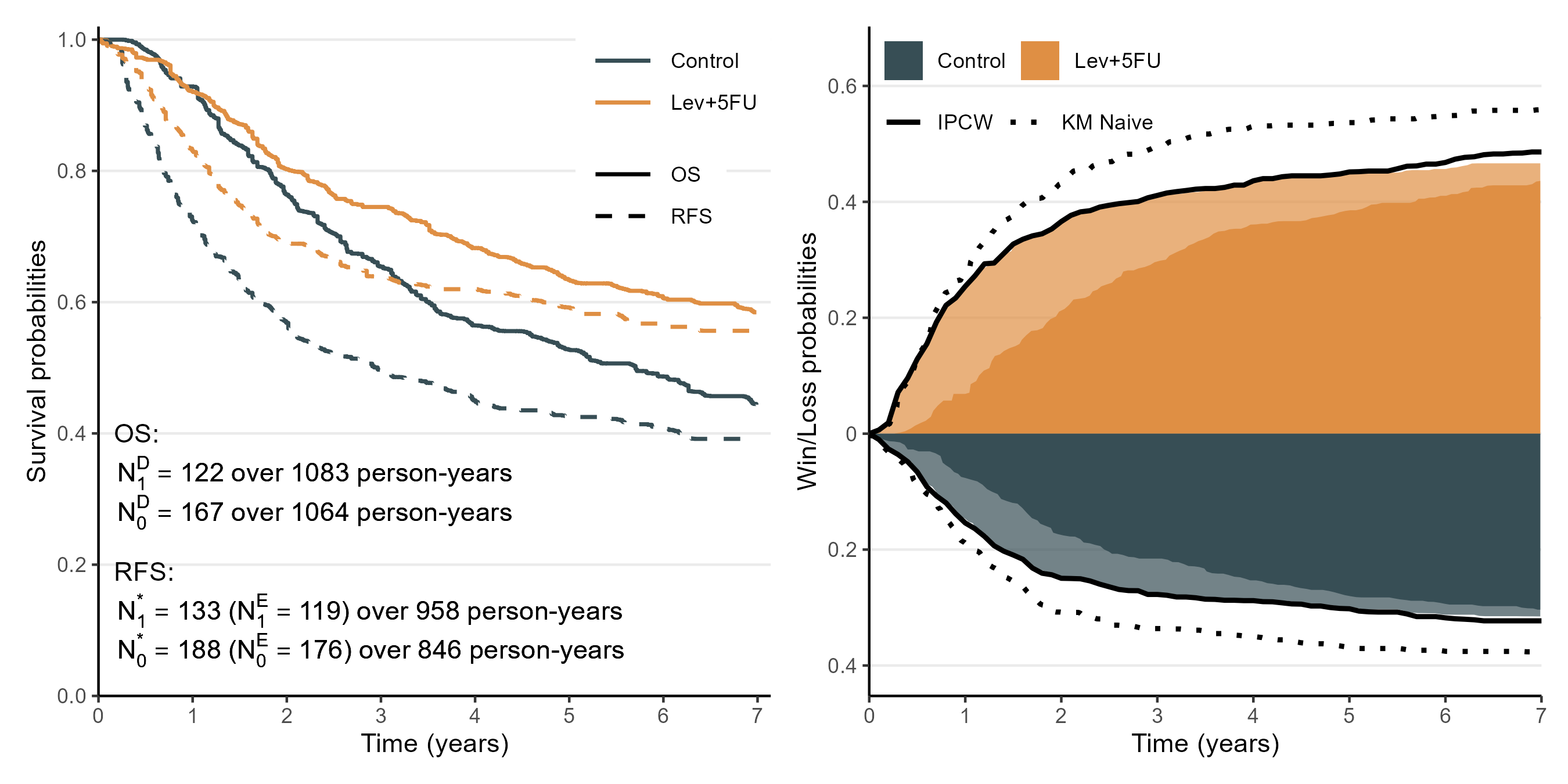
Colon Cancer Trial
- Stage C disease (Moertel et al., 1990)
- Combined treatment (Lev+5FU; \(n=304\)) vs control (\(n=314\) patients)
- KM curves for OS and relapse-free survival (RFS)
- Extract estimates \(\hat{S}_a(t)\) and \(\hat{S}_a^*(t)\) from graphs using WebPlotDigitizer
- Total event counts and person-years of follow-up from paper
- Compare estimates of \(w_{1,0}(\tau)\) and \(w_{0,1}(\tau)\)
- Adjusting for association between death and relapse (area plot)
- KM naive: without adjustment
- IPCW (reference): raw data-based estimates (Dong et al., 2020; Parner & Overgaard, 2024)
Colon Cancer Trial: Results
- Left: summary data; right: approximation results
- 1-, 2-, 4-, and 7-year win ratios by the adjusted method (comparing with IPCW): 1.71 (1.65), 1.47 (1.47), 1.53 (1.51), and 1.48 (1.51), respectively
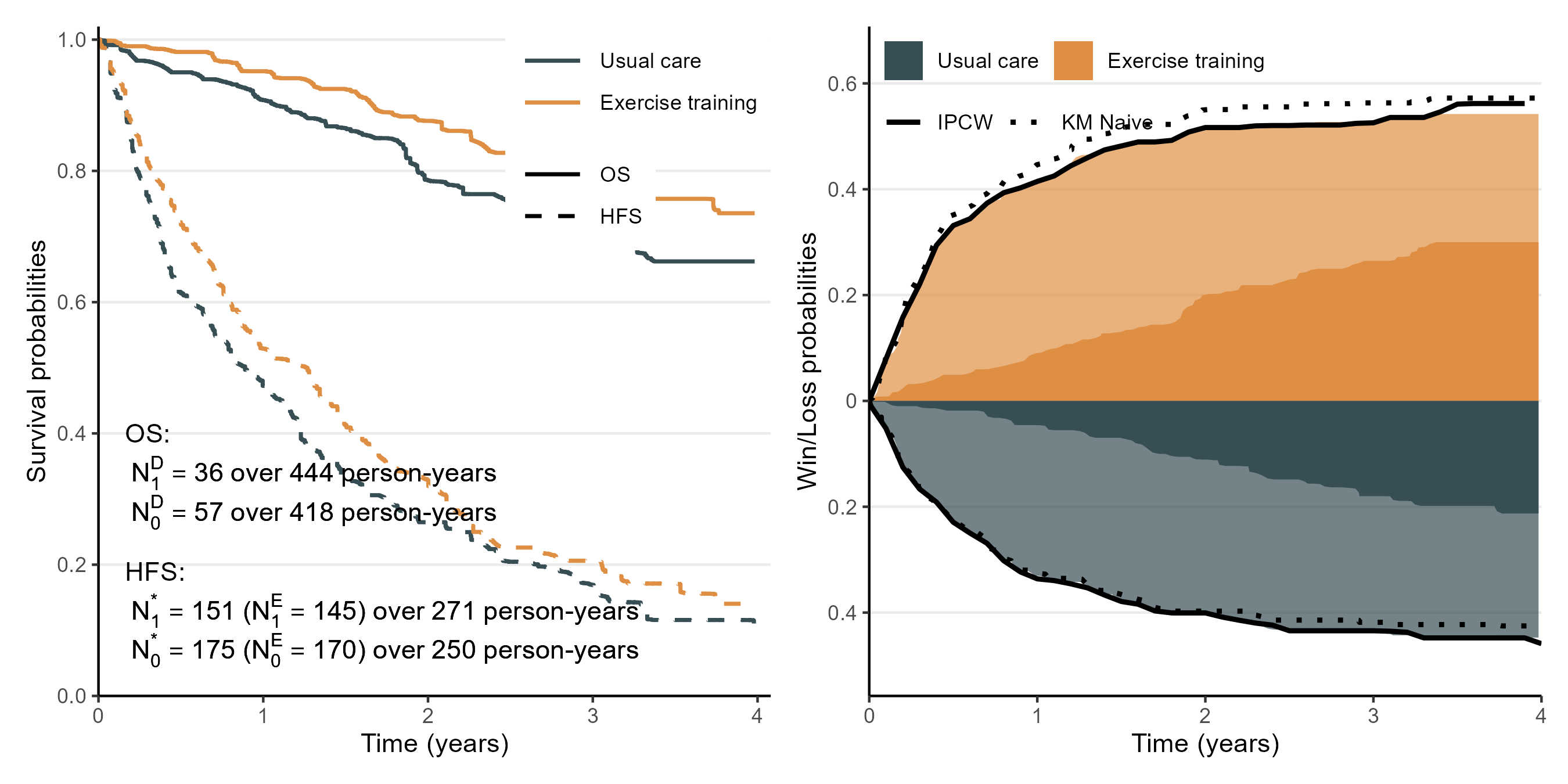
HF-ACTION Trial
- Study background (O’Connor et al., 2009)
- 2,000+ heart failure patients from North America and France
- Non-ischemic patients with baseline cardiopulmonary exercise test lasting 9 minutes or less (426 patients)
- Exercise training (\(n=205\)) vs usual care (\(n=221\))
- KM curves for OS and hospitalization-free survival (HFS)
- Extract estimates \(\hat{S}_a(t)\) and \(\hat{S}_a^*(t)\) from graphs using WebPlotDigitizer
- Total event counts and person-years of follow-up from paper
HF-ACTION Trial: Results
- Left: summary data; right: approximation results
- 1-, 2-, 3-, and 4-year win ratios by the adjusted method (comparing with IPCW): 1.27 (1.23), 1.27 (1.29), 1.21 (1.21), and 1.21 (1.26), respectively
Conclusion
Additional Resources
Manuscript
Mao, L. (2025+) Approximating Win-Loss Probabilities Based on the Overall and Event-Free Survival Functions. Available at http://dx.doi.org/10.2139/ssrn.5142445
WinKMWebsiteCalculating win-loss statistics using summary data: https://lmaowisc.github.io/winkm/
Summary and Future Work
WinKM: approximating win-loss measures using published OS and EFS data- Scanned KM curves
- Event counts (deaths, EFS endpoints, nonfatal events)
- Total follow-up times (from risk tables)
- Adding standard errors
- Optimal combination of study-specific effect sizes
- Assessment of between-study heterogeneities