Tidy Survival Analysis: Applying R’s Tidyverse to Survival Data
Module 5. Machine Learning
Lu Mao
Department of Biostatistics & Medical Informatics
University of Wisconsin-Madison
Aug 3, 2025
Machine Learning Survival Models
Setting
- With many covariates
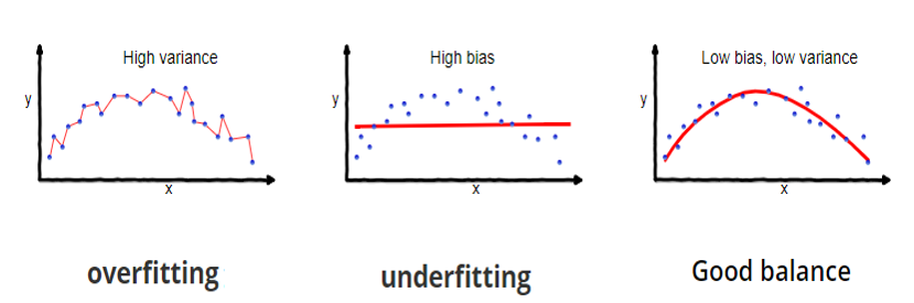
- Prediction accuracy: under- vs over-fitting
![]()
- Too many predictors \(\to\) overfitting
- Interpretation: easier with fewer predictors
- Prediction accuracy: under- vs over-fitting
Regularized Cox Regression
- Idea
- Penalize the magnitude of coefficients (\(L^q\)-norm) to avoid overfitting
- Elastic net: minimize objective function \[
\ell(\beta) = -\mbox{log-partial-likelihood}(\beta) + \lambda\sum_{j=1}^p\left\{\alpha|\beta_j|+2^{-1}(1-\alpha)\beta_j^2\right\}
\]
- \(\lambda\): tuning parameter that controls the strength of penalty
- Determined by cross-validation
- \(\alpha\): controls the type of penalty
- \(\alpha = 0\) \(\to\) ridge regression: handles correlated predictors better
- \(\alpha = 1\) \(\to\) lasso regression: performs variable selection
- Implementation:
glmnetpackage
- \(\lambda\): tuning parameter that controls the strength of penalty
Survival Trees
- Decision trees
- Classification and Regression Trees (CART; Breiman et al., 1984)
- Root node (all sample) \(\stackrel{\rm covariates}{\rightarrow}\) split into (more homogeneous) daughter nodes \(\stackrel{\rm covariates}{\rightarrow}\) split recursively
- Growing the tree
- Starting with root node, search partition criteria \[Z_{\cdot j}\leq z \,\,\,(j=1,\ldots, p; z \in\mathbb R)\] for one that minimizes “impurity” (e.g., mean squared deviance residuals) within daughter nodes \[\begin{equation}\label{eq:tree:nodes} A=\{i=1,\ldots, n: Z_{ij}\leq z\} \mbox{ and } B=\{i=1,\ldots, n: Z_{ij}> z\} \end{equation}\]
- Recursive splitting until terminal nodes sufficiently “pure” in outcome
Complexity Control and Prediction
- Pruning the tree
- Cut overgrown branches to prevent overfitting
- Penalize number of terminal nodes
- Tune complexity parameter (or minimum size of terminal node)
- Prediction
- New \(z\) \(\rightarrow\) terminal node \(\rightarrow\) KM estimates (or median survival)
- Implementation:
rpartpackage
Random Forests
- Limitation of a single tree
- High variance: small changes in data can lead to large changes in predictions
- Random forests
- Bootstrap samples from training data
- Take a random subset of covariates to split on (decorrelate the trees)
- Tune the number of covariates to split on
- Implementation:
aorsfpackage
Model Evaluation
- Brier score
- Mean squared error between observed survival status and predicted survival probability
- Inverse probability censoring weighting (IPCW) to account for censoring
- Integrated Brier score: average Brier score over a time interval
- ROC AUC
- Area under the receiver operating characteristic (ROC) curve for survival status
- IPCW to handle censoring
- Concordance index: overall AUC over time
tidymodels Workflows
Overview of tidymodels and censored
tidymodels: a collection of packages for modeling and machine learning in R- Provides a consistent interface for model training, tuning, and evaluation
- Key package
parsnip
- Key package
- Supports various model types, including regression, classification, and survival analysis
- Provides a consistent interface for model training, tuning, and evaluation
censored: aparsnipextension package for survival data- Implements parametric, semiparametric, and tree-based survival models
Data Preparation and Splitting
- Create a
Survobject as responseSurv(time, event)
Data splitting
initial_split(): splits data into training and testing sets
Model Specification
- Model type
survival_reg(): parametric AFT modelsproportional_hazards(penalty = tune()): (regularized) Cox PH modelsdecision_tree(cost_complexity = tune()): decision treesrand_forest(mtry = tune()): random forests
- Set engine and mode
set_engine("survival"): for AFT modelsset_engine("glmnet"): for Cox PH modelsset_engine("aorsf"): for random forestsset_mode("censored regression"): for survival models
Recipe and Workflow
- Recipe: a series of preprocessing steps for the data
recipe(response ~ ., data = df): specify response and predictorsstep_mutate(): standardize numeric predictorsstep_dummy(): convert categorical variables to dummy variables
- Workflow: combines model specification and recipe
workflow() |> add_model(model_spec) |> add_recipe(recipe)
# Create a recipe
model_recipe <- recipe(surv_obj ~ ., data = df_train) |> # specify formula
  step_mutate(z1 = z1 / 1000) |>  # standardize z1
  step_other(z2, z3, threshold = 0.02) |> # group levels with prop < .02 into "other"
  step_dummy(all_nominal_predictors())  # convert categorical variables to dummy variables
# Create a workflow by combining model and recipe
model_wflow <- workflow() |>
  add_model(model_spec) |>   # add model specification
  add_recipe(model_recipe)   # add recipe
Tune Hyperparameters
- Cross-validation
df_train_folds <- vfold_cv(df_train, v = k): create k-folds on training data (default 10)tune_grid(model_wflow, resamples = df_train_folds): tune hyperparameters using cross-validation
# k-fold cross-validation
df_train_folds <- vfold_cv(df_train, v = 10) # 10-fold cross-validation
# Tune hyperparameters
model_res <- tune_grid(
  model_wflow,
  resamples = df_train_folds,
  grid = 10, # number of hyperparameter combinations to try
  metrics = metric_set(brier_survival, brier_survival_integrated,  # specify metrics
                       roc_auc_survival, concordance_survival),
  eval_time = seq(0, 84, by = 12) # evaluation time points
)
Finalize Workflow
- Examine validation results
collect_metrics(model_res): collect metrics from tuning resultsshow_best(model_res, metric = "brier_survival_integrated", n = 5): show top 5 models based on Brier score
- Workflow for best model
param_best <- select_best(model_res, metric = "brier_survival_integrated"): select best hyperparameters based on Brier scorefinal_wl <- finalize_workflow(model_wflow, param_best): finalize workflow with best hyperparameters
Fit Final Model
- Fit the finalized workflow
final_mod <- last_fit(final_wl, split = df_split): fit the finalized workflow on the testing setcollect_metrics(final_mod): collect metrics of final model on test data
- Make predictions
predict(final_mod, new_data = new_data, type = "time"): predict survival times on new data
# Fit the finalized workflow on the testing set
final_mod <- last_fit(final_wl, split = df_split)
# Collect metrics of final model on test data
collect_metrics(final_mod) %>%
  filter(.metric == "brier_survival_integrated")
# Make predictions on new data
new_data <- testing(df_split) |>  slice(1:5) # take first 5 rows of test data
predict(final_mod, new_data = new_data, type = "time")
A Case Study
GBC: Relapse-Free Survival
- Time to first event
library(tidymodels) # load tidymodels
library(censored)
gbc <- read.table("data/gbc.txt", header = TRUE) # Load GBC dataset
df <- gbc |>  # calculate time to first event (relapse or death)
  group_by(id) |> # group by id
  arrange(time) |> # sort rows by time
  slice(1) |>      # get the first row within each id
  ungroup() |>
  mutate(
    surv_obj = Surv(time, status), # create the Surv object as response variable
    .after = id, # keep id column after surv_obj
    .keep = "unused" # discard original time and status columns
  )
Data Preparation
- Analysis dataset
# A tibble: 6 × 10
     id   surv_obj hormone   age  meno  size grade nodes  prog estrg
  <int>     <Surv>   <int> <int> <int> <int> <int> <int> <int> <int>
1     1 43.836066        1    38     1    18     3     5   141   105
2     2 46.557377        1    52     1    20     1     1    78    14
3     3 41.934426        1    47     1    30     2     1   422    89
4     4  4.852459+       1    40     1    24     1     3    25    11
5     5 61.081967+       2    64     2    19     2     1    19     9
6 6 63.377049+ 2 49 2 56 1 3 356 64- Data splitting
Models to be Trained
- Regularized Cox model
proportional_hazards(penalty = tune())- Default: \(\alpha = 1\) (lasso)
- Tune penalty parameter \(\lambda\)
- Use
glmnetengine for fitting
- Random forest
rand_forest(mtry = tune(), min_n = tune())- Tune number of predictors to split on and minimum size of terminal node
- Use
aorsfengine for fitting
Common Recipe
- Recipe for both models
gbc_recipe <- recipe(surv_obj ~ ., data = gbc_train) |> # specify formula
  step_mutate(
    grade = factor(grade),
    age40 = as.numeric(age >= 40), # create a binary variable for age >= 40
    prog = prog / 100, # rescale prog
    estrg = estrg / 100 # rescale estrg
  ) |>
  step_dummy(grade) |>
  step_rm(id) # remove id
# gbc_recipe # print recipe information
Regularized Cox Model
- Cox model specification and workflow
# Regularized Cox model specification
cox_spec <- proportional_hazards(penalty = tune()) |>  # tune lambda
  set_engine("glmnet") |>  # set engine to glmnet
  set_mode("censored regression") # set mode to censored regression
cox_spec # print model specification
Proportional Hazards Model Specification (censored regression)
Main Arguments:
penalty = tune()
Computational engine: glmnet Model Tuning
- Cross-validation set-up
- For both models
set.seed(123) # set seed for reproducibility
gbc_folds <- vfold_cv(gbc_train, v = 10) # 10-fold cross-validation
# Set evaulation metrics
gbc_metrics <- metric_set(brier_survival, brier_survival_integrated,
                          roc_auc_survival, concordance_survival)
gbc_metrics # evaluation metrics info
A metric set, consisting of:
- `brier_survival()`, a dynamic survival metric | direction:
minimize
- `brier_survival_integrated()`, a integrated survival metric | direction:
minimize
- `roc_auc_survival()`, a dynamic survival metric | direction:
maximize
- `concordance_survival()`, a static survival metric | direction:
maximizeCox Model Tuning
- Tune the regularized Cox model
- Use
tune_grid()to perform hyperparameter tuning - Evaluate performance using Brier score and ROC AUC
- Use
set.seed(123) # set seed for reproducibility
# Tune the regularized Cox model (this will take some time)
cox_res <- tune_grid(
  cox_wflow,
  resamples = gbc_folds,
  grid = 10, # number of hyperparameter combinations to try
  metrics = gbc_metrics, # evaluation metrics
  eval_time = time_points, # evaluation time points
  control = control_grid(save_workflow = TRUE) # save workflow
)
Cox Model Tuning Results
- Plot Brier score as function of \(\log\lambda\)
collect_metrics(cox_res) |>  # collect metrics from tuning results
  filter(.metric == "brier_survival_integrated") |>  # filter for Brier score
  ggplot(aes(log(penalty), mean)) + # plot log-lambda vs Brier score
  geom_line() +  # plot line
  labs(x = "Log-lambda", y = "Overall Brier Score") + # labels
  theme_classic() # classic theme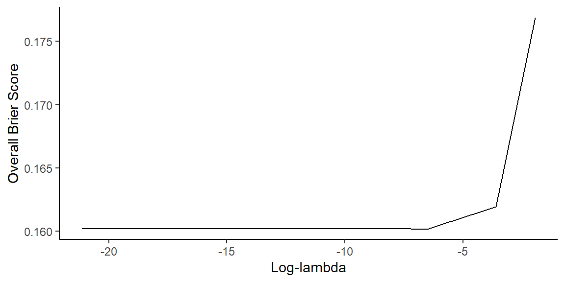
Best Cox Models
Show best models
- Based on Brier score
# A tibble: 5 × 8
       penalty .metric         .estimator .eval_time  mean     n std_err .config
         <dbl> <chr>           <chr>           <dbl> <dbl> <int>   <dbl> <chr>
1 0.00147      brier_survival… standard           NA 0.160    10 0.00775 Prepro…
2 0.0000127    brier_survival… standard           NA 0.160    10 0.00775 Prepro…
3 0.0000000105 brier_survival… standard           NA 0.160    10 0.00775 Prepro…
4 0.000754     brier_survival… standard           NA 0.160    10 0.00775 Prepro…
5 0.00000409   brier_survival… standard           NA 0.160    10 0.00775 Prepro…
Random Forest Model
- Random forest specification and workflow
# Random forest model specification
rf_spec <- rand_forest(mtry = tune(), min_n = tune()) |>  # tune mtry and min_n
  set_engine("aorsf") |>  # set engine to aorsf
  set_mode("censored regression") # set mode to censored regression
rf_spec # print model specification
Random Forest Model Specification (censored regression)
Main Arguments:
mtry = tune()
min_n = tune()
Computational engine: aorsf Random Forest Tuning
- Tune the random forest model
- Similar to Cox model tuning
set.seed(123) # set seed for reproducibility
# Tune the random forest model (this will take some time)
rf_res <- tune_grid(
  rf_wflow,
  resamples = gbc_folds,
  grid = 10, # number of hyperparameter combinations to try
  metrics = gbc_metrics, # evaluation metrics
  eval_time = time_points # evaluation time points
)
Random Forest Tuning Results
- View validation results
# A tibble: 6 × 9
   mtry min_n .metric         .estimator .eval_time   mean     n std_err .config
  <int> <int> <chr>           <chr>           <dbl>  <dbl> <int>   <dbl> <chr>
1     3    30 brier_survival  standard            0 0         10 0       Prepro…
2     3    30 roc_auc_surviv… standard            0 0.5       10 0       Prepro…
3     3    30 brier_survival  standard           12 0.0635    10 0.00706 Prepro…
4     3    30 roc_auc_surviv… standard           12 0.827     10 0.0314  Prepro…
5     3    30 brier_survival  standard           24 0.163     10 0.0114  Prepro…
6     3    30 roc_auc_surviv… standard           24 0.747     10 0.0475  Prepro…
Best Random Forest Models
- Show best models
- Based on Brier score
# A tibble: 5 × 9
   mtry min_n .metric          .estimator .eval_time  mean     n std_err .config
  <int> <int> <chr>            <chr>           <dbl> <dbl> <int>   <dbl> <chr>
1     6    24 brier_survival_… standard           NA 0.155    10 0.00765 Prepro…
2     5    27 brier_survival_… standard           NA 0.155    10 0.00782 Prepro…
3     4    20 brier_survival_… standard           NA 0.156    10 0.00777 Prepro…
4     9    36 brier_survival_… standard           NA 0.156    10 0.00743 Prepro…
5 2 7 brier_survival_… standard NA 0.156 10 0.00829 Prepro…- Conclusion
- Best RF model has lower Brier score than best Cox model
Finalize and Fit Best Model
- Fit final RF model
# Select best RF hyperparameters (mtry, min_n) based on Brier score
param_best <- select_best(rf_res, metric = "brier_survival_integrated")
param_best # view results
# A tibble: 1 × 3
mtry min_n .config
<int> <int> <chr>
1 6 24 Preprocessor1_Model07# Finalize the workflow with the best hyperparameters
rf_final_wflow <- finalize_workflow(rf_wflow, param_best) # finalize workflow
# Fit the finalized workflow on the testing set
set.seed(123) # set seed for reproducibility
final_rf_fit <- last_fit(
rf_final_wflow,
split = gbc_split, # use the original split
metrics = gbc_metrics, # evaluation metrics
eval_time = time_points # evaluation time points
)Test Performance (I)
- Collect metrics on test data
collect_metrics(final_rf_fit) |> # collect overall performance metrics
  filter(.metric %in% c("concordance_survival", "brier_survival_integrated"))
# A tibble: 2 × 5
.metric .estimator .eval_time .estimate .config
<chr> <chr> <dbl> <dbl> <chr>
1 brier_survival_integrated standard NA 0.237 Preprocessor1_Model1
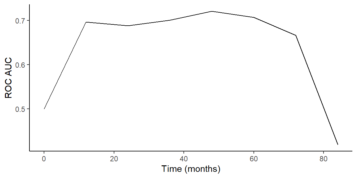
2 concordance_survival standard NA 0.655 Preprocessor1_Model1Test Performance (II)
- Plot test ROC AUC over time
Prediction by Final RF Model
- Extract the fitted workflow
- Use
extract_workflow()to get the final model
- Use
gbc_rf <- extract_workflow(final_rf_fit) # extract the fitted workflow
# Predict on new data
gbc_5 <- testing(gbc_split) |>  slice(1:5) # take first 5 rows of test data
predict(gbc_rf, new_data = gbc_5, type = "time") # predict survival times
# A tibble: 5 × 1
.pred_time
<dbl>
1 47.6
2 67.1
3 67.2
4 36.1
5 49.7Cox Model Exercise (I)
- Task: extract the best Cox model from
cox_resand fit it to test data
Solution
# Select best Cox hyperparameters (penalty) based on Brier score
param_best_cox <- select_best(cox_res, metric = "brier_survival_integrated")
# Finalize the workflow with the best hyperparameters
cox_final_wflow <- finalize_workflow(cox_wflow, param_best_cox) # finalize workflow
# Fit finalized workflow on the testing set
final_cox_fit <- last_fit(
  cox_final_wflow,
  split = gbc_split, # use the original split
  metrics = gbc_metrics, # evaluation metrics
  eval_time = time_points # evaluation time points
)
# Collect metrics on test data
collect_metrics(final_cox_fit) |> # collect overall performance metrics
  filter(.metric %in% c("concordance_survival", "brier_survival_integrated"))
Cox Model Exercise (II)
Solution - continued
# Extract test ROC AUC over time
roc_test_cox <- collect_metrics(final_cox_fit) |>
  filter(.metric == "roc_auc_survival") |>  # filter for ROC AUC
  rename(mean = .estimate) # rename mean column
roc_test_cox |>  # pass the test ROC AUC data
  ggplot(aes(.eval_time, mean)) +  # plot evaluation time vs mean ROC AUC
  geom_line() + # plot line
  labs(x = "Time (months)", y = "ROC AUC") + # labels
  theme_classic()

# Predict on new data
# Extract fitted workflow
gbc_cox <- extract_workflow(final_cox_fit) # extract the fitted workflow
gbc_5 <- testing(gbc_split) |>  slice(1:5) # take first 5 rows of test data
predict(gbc_cox, new_data = gbc_5, type = "time") # predict survival times
Cox Model Exercise (III)
- Task: find the parameter estimates of final Cox model
- Hint: use
tidy()function frombroompackage
- Hint: use
Solution
tidy(gbc_cox) # tidy the coefficients
# # A tibble: 10 × 3
#    term     estimate penalty
#    <chr>       <dbl>   <dbl>
#  1 hormone  -0.227   0.00147
#  2 age       0.00908 0.00147
#  3 meno     -0.00736 0.00147
#  4 size      0.0127  0.00147
#  5 nodes     0.0411  0.00147
#  6 prog     -0.270   0.00147
#  7 estrg     0.00771 0.00147
#  8 age40    -0.540   0.00147
#  9 grade_X2  0.573   0.00147
# 10 grade_X3  0.624   0.00147
Survival Tree Exercise
- Task: fit a survival tree model to the GBC data
- Use
decision_tree()withset_engine("rpart") - Tune complexity parameter
cost_complexityusingtune() - Use the same recipe as for Cox and RF models
- Evaluate performance using Brier score and ROC AUC
- Use
Summary
Key Takeaways
- Machine learning: powerful tools for survival analysis with many covariates
- Regularized Cox regression, survival trees, and random forests
tidymodels: a consistent interface for modeling and machine learningparsnipfor model specification and tuningcensoredpackages for survival data- Model evaluation: Brier score and ROC AUC for survival models