Tidy Survival Analysis: Applying R’s Tidyverse to Survival Data

Module 4. Semiparametric Regression Analysis

Lu Mao

lmao@biostat.wisc.edu

Department of Biostatistics & Medical Informatics

University of Wisconsin-Madison

Aug 3, 2025

Presenting Regression Results

Cox PH Regression

Model specification \[ \lambda(t \mid Z) = \lambda_0(t) \exp(\beta_1 Z_1 + \beta_2 Z_2 + \ldots + \beta_p Z_p) \]
- \(\lambda_0(t)\): baseline hazard function
- \(\exp(\beta_j)\): hazard ratio for covariate \(Z_j\)
GBC data: relapse-free survival

library(tidyverse) # Load tidyverse packages
gbc <- read.table("data/gbc.txt", header = TRUE) # Load GBC dataset

GBC Data: a Running Example

Reformat the data

df <- gbc |>  # calculate time to first event (relapse or death)
  group_by(id) |> # group by id
  arrange(time) |> # sort rows by time
  slice(1) |>      # get the first row within each id
  ungroup() |>     # remove grouping
  mutate(
    age40 = ifelse(age >= 40, 1, 0), # create binary variable for age >= 40
    grade = factor(grade), # convert grade to factor
    prog = prog / 100, # rescale progesterone receptor
    estrg = estrg / 100 # rescale estrogen receptor
    )

Analysis in Base R

Model fitting: survival::coxph()

library(survival) # Load survival package
cox_fit <- coxph(Surv(time, status) ~ hormone + meno + age40 + grade + size + prog + estrg, 
                 data = df)
summary(cox_fit) # Print model summary

Call:
coxph(formula = Surv(time, status) ~ hormone + meno + age40 + 
    grade + size + prog + estrg, data = df)

  n= 686, number of events= 299 

            coef exp(coef) se(coef)      z Pr(>|z|)    
hormone -0.37432   0.68776  0.12917 -2.898 0.003758 ** 
meno     0.28450   1.32909  0.13973  2.036 0.041748 *  
age40   -0.55127   0.57622  0.20243 -2.723 0.006463 ** 
grade2   0.71547   2.04514  0.24854  2.879 0.003993 ** 
grade3   0.77465   2.16982  0.26970  2.872 0.004075 ** 
size     0.01606   1.01619  0.00368  4.365 1.27e-05 ***
prog    -0.22400   0.79932  0.05776 -3.878 0.000105 ***
estrg    0.01204   1.01212  0.04680  0.257 0.796895    
---
Signif. codes:  0 '***' 0.001 '**' 0.01 '*' 0.05 '.' 0.1 ' ' 1

        exp(coef) exp(-coef) lower .95 upper .95
hormone    0.6878     1.4540    0.5339    0.8859
meno       1.3291     0.7524    1.0107    1.7478
age40      0.5762     1.7355    0.3875    0.8568
grade2     2.0451     0.4890    1.2565    3.3287
grade3     2.1698     0.4609    1.2790    3.6812
size       1.0162     0.9841    1.0089    1.0236
prog       0.7993     1.2511    0.7138    0.8951
estrg      1.0121     0.9880    0.9234    1.1093

Concordance= 0.661  (se = 0.016 )
Likelihood ratio test= 78.79  on 8 df,   p=9e-14
Wald test            = 68.82  on 8 df,   p=8e-12
Score (logrank) test = 69.51  on 8 df,   p=6e-12

Tidy `coxph()` Output

Using broom package: broom::tidy()
- Provides a tidy data frame for easy manipulation and visualization

library(broom) # Load broom package
tidy_cox <- tidy(cox_fit) # Tidy the coxph output
tidy_cox # Display the tidy output

# A tibble: 8 × 5
  term    estimate std.error statistic   p.value
  <chr>      <dbl>     <dbl>     <dbl>     <dbl>
1 hormone  -0.374    0.129      -2.90  0.00376  
2 meno      0.284    0.140       2.04  0.0417   
3 age40    -0.551    0.202      -2.72  0.00646  
4 grade2    0.715    0.249       2.88  0.00399  
5 grade3    0.775    0.270       2.87  0.00408  
6 size      0.0161   0.00368     4.37  0.0000127
7 prog     -0.224    0.0578     -3.88  0.000105 
8 estrg     0.0120   0.0468      0.257 0.797

Tabulating Results with `gtsummary` (I)

Using gtsummary package: tbl_regression()
- Automatically formats regression results into a publication-ready table

library(gtsummary) # Load gtsummary package
cox_tbl <- cox_fit |> tbl_regression( # Create a regression table
                exponentiate = TRUE, # Exponentiate coefficients to get hazard ratios
                label = list(hormone ~ "Hormone Therapy", # Custom labels
                             meno ~ "Menopausal", 
                             age40 ~ "Older than 40", 
                             grade ~ "Tumor Grade", 
                             size ~ "Tumor Size (mm)", 
                             prog ~ "Progesterone Receptor (100 fmol/ml)", 
                             estrg ~ "Estrogen Receptor  (100 fmol/ml)")
               ) |> 
          add_global_p() # Add global p-value for categorical variables
cox_tbl # Display the regression table

Tabulating Results with `gtsummary` (II)

Result

Characteristic	HR¹	95% CI¹	p-value
Hormone Therapy	0.69	0.53, 0.89	0.003
Menopausal	1.33	1.01, 1.75	0.039
Older than 40	0.58	0.39, 0.86	0.009
Tumor Grade			0.004
1	—	—
2	2.05	1.26, 3.33
3	2.17	1.28, 3.68
Tumor Size (mm)	1.02	1.01, 1.02	<0.001
Progesterone Receptor (100 fmol/ml)	0.80	0.71, 0.90	<0.001
Estrogen Receptor (100 fmol/ml)	1.01	0.92, 1.11	0.8
¹ HR = Hazard Ratio, CI = Confidence Interval

Further Customization

Styling functions
- modify_header(): update column headers
- modify_footnote_header(): update column header footnote
- modify_footnote_body(): update table body footnote
- modify_caption(): update table caption/title
- bold_labels(): bold variable labels
- bold_levels(): bold variable levels
- italicize_labels(): italicize variable labels
- italicize_levels(): italicize variable levels
- bold_p(): bold significant p-values
More about tbl_regression()
- gtsummary documentation

Table Customization Exercise

Task: Customize the regression table
- Add a caption: “Cox regression analysis of the German breast cancer study”
- Bold significant p-values
- Italicize tumor grade levels

Solution

cox_tbl |> # Start with the regression table
  modify_caption("Cox regression analysis of the German breast cancer study") |> # Add caption
  bold_p() |> # Bold significant p-values
  italicize_levels() # Italicize variable levels

Other Regression Models

Accelerated failure time (AFT) models \[ \log T = \beta_1 Z_1 + \beta_2 Z_2 + \ldots + \beta_p Z_p + \epsilon \]
- \(\epsilon\sim\) Weibull, lognormal, etc. (parametric models)
- \(\exp(\beta_j)\): acceleration factor for covariate \(Z_j\)
- Model fitting: survival::survreg()

# Fit a Weibull AFT model
aft_fit <- survreg(Surv(time, status) ~ hormone + meno + age + grade + size + prog + estrg, 
                    data = df, dist = "weibull") # specify the Weibull model

Exercise

Tidy up the survreg object aft_fit using broom::tidy()
Create a regression table using gtsummary::tbl_regression()

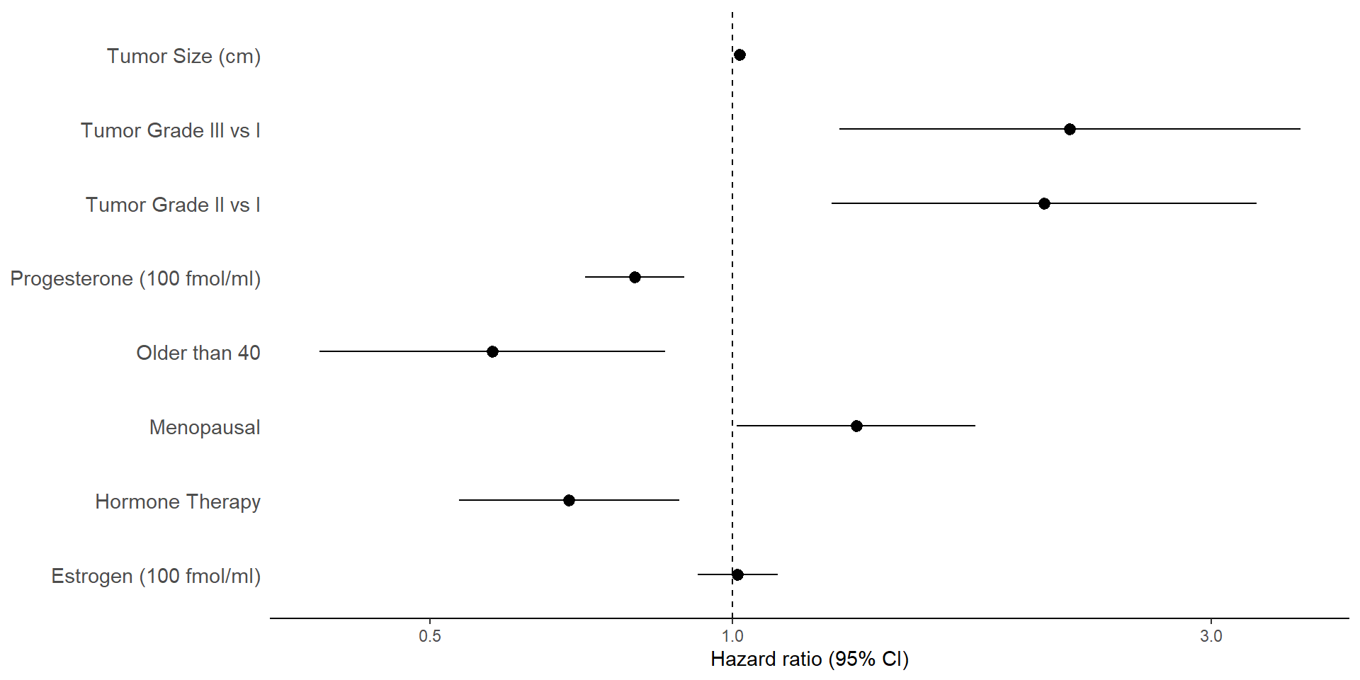
Visualizing Hazard Ratios (I)

Forest plot: Visualize hazard ratios and confidence intervals

# Tidy with exponentiated coeffs (HR) and CI
tidy_cox <- tidy(cox_fit, exponentiate = TRUE, conf.int = TRUE) 
tidy_cox$term <- recode(tidy_cox$term,           # Relabel the variables
                hormone = "Hormone Therapy", 
                meno = "Menopausal", 
                age40 = "Older than 40", 
                grade2 = "Tumor Grade II vs I",
                grade3 = "Tumor Grade III vs I",
                size = "Tumor Size (mm)", 
                prog = "Progesterone (100 fmol/ml)", 
                estrg = "Estrogen (100 fmol/ml)")

tidy_cox |>  # plot of hazard ratios and 95% CIs
  ggplot(aes(y=term, x=estimate, xmin=conf.low, xmax=conf.high)) + 
  geom_pointrange() +  # plots center point (x) and range (xmin, xmax)
  geom_vline(xintercept=1, linetype = 2) + # vertical line at HR=1
  scale_x_log10("Hazard ratio (95% CI)") + # log scale for x-axis
  theme_classic() + # classic theme for clean look
  theme(
    axis.line.y = element_blank(),          # remove y-axis line
    axis.ticks.y = element_blank(),         # remove y-axis ticks
    axis.text.y = element_text(size = 11),  # set variable label size
    axis.title.y = element_blank()          # remove y-axis title
  )

Visualizing Hazard Ratios (II)

Result

Forest Plot Exercise

Task: customize the forest plot
- Use square rather than default circle for point estimates
- Set x-axis ticks at 0.5, 1, 2.0, and 4.0
- Add a title: “Cox Regression Results for GBC Data”

Solution

tidy_cox |> 
  ggplot(aes(y=term, x=estimate, xmin=conf.low, xmax=conf.high)) + 
  geom_pointrange(shape = 15) +  # plots center point (x) in square and range (xmin, xmax)
  geom_vline(xintercept=1, linetype = 2) + # vertical line at HR=1
  scale_x_log10("Hazard ratio (95% CI)",    # log scale for x-axis
                breaks = c(0.5, 1, 2, 4)) + # log scale for x-axis
  ggtitle("Cox Regression Results for GBC Data") + # Add title
  theme_classic() + # classic theme for clean look
  theme(
    axis.line.y = element_blank(),          # remove y-axis line
    axis.ticks.y = element_blank(),         # remove y-axis ticks
    axis.text.y = element_text(size = 11),  # set variable label size
    axis.title.y = element_blank()          # remove y-axis title
  )

Cox Model Prediction and Diagnostics

Model-Based Prediction

Predicted survival function \[ \hat S(t \mid z) = \exp\left\{- \exp(\hat\beta^\mathrm{T} z) \hat\Lambda_0(t)\right\} \]

Prepare new data for prediction

A post-menpausal woman older than 40, undergoing hormone therapy, with tumor grade II, tumor size 20 mm, and progesterone and estrogen receptor levels both 100 fmol/ml.

# Create new data for prediction
# specify all covariate values
new_data <- data.frame(hormone = 2, meno = 2, age40 = 1, grade = factor(2), 
                        size = 20, prog = 1, estrg = 1)

new_data

  hormone meno age40 grade size prog estrg
1       2    2     1     2   20    1     1

Tidy Survival Prediction

Use survival::survfit() to predict survival probabilities

newdata: new data for prediction
times: time points for prediction
broom::tidy() to tidy the output

# Predict survival probabilities for `newdata`
pred_surv <- survfit(cox_fit, newdata = new_data[1, ])
tidy_pred_surv <- tidy(pred_surv) # Tidy the survival prediction output
head(tidy_pred_surv) # Display the first few rows of the tidy output

# A tibble: 6 × 8
   time n.risk n.event n.censor estimate std.error conf.high conf.low
  <dbl>  <dbl>   <dbl>    <dbl>    <dbl>     <dbl>     <dbl>    <dbl>
1 0.262    686       0        1        1         0         1        1
2 0.492    685       0        1        1         0         1        1
3 0.525    684       0        1        1         0         1        1
4 0.557    683       0        2        1         0         1        1
5 0.590    681       0        1        1         0         1        1
6 0.951    680       0        1        1         0         1        1

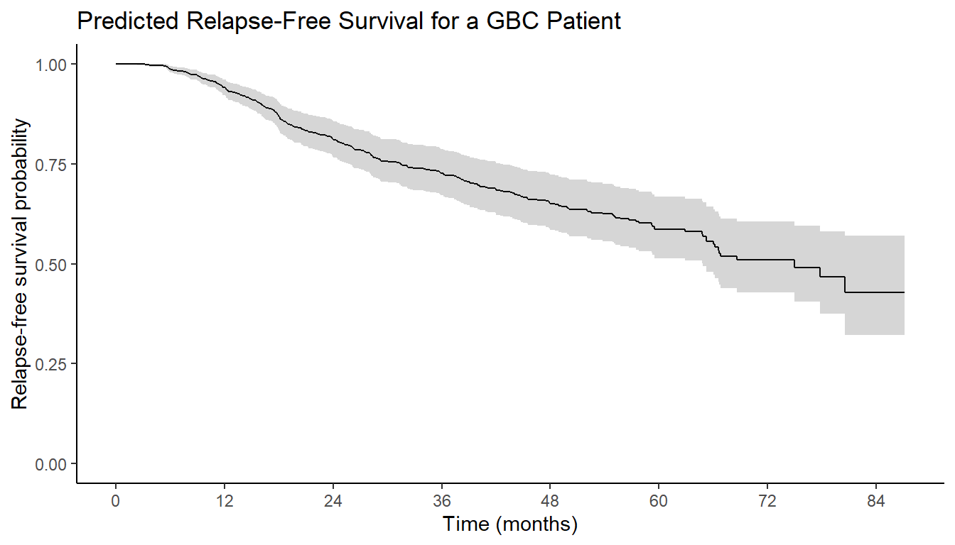
Visualizing Predicted Survival (I)

Using ggsurvfit package: ggsurvfit()
- Pass survfit object to ggsurvfit()
- Similar customization to KM curves

library(ggsurvfit) # Load ggsurvfit package
pred_fig <- pred_surv |>  # Pass the survfit object
  ggsurvfit() + # Main function
  add_confidence_interval() + # Add confidence interval
  scale_x_continuous("Time (months)", breaks = seq(0, 84, by = 12)) + # x-axis format
  scale_y_continuous("Relapse-free survival probability", limits = c(0, 1)) + # y-axis format
  ggtitle("Predicted Relapse-Free Survival for a GBC Patient") + # Add title
  theme_classic() # Classic theme for clean look

Visualizing Predicted Survival (II)

Result

pred_fig # print figure

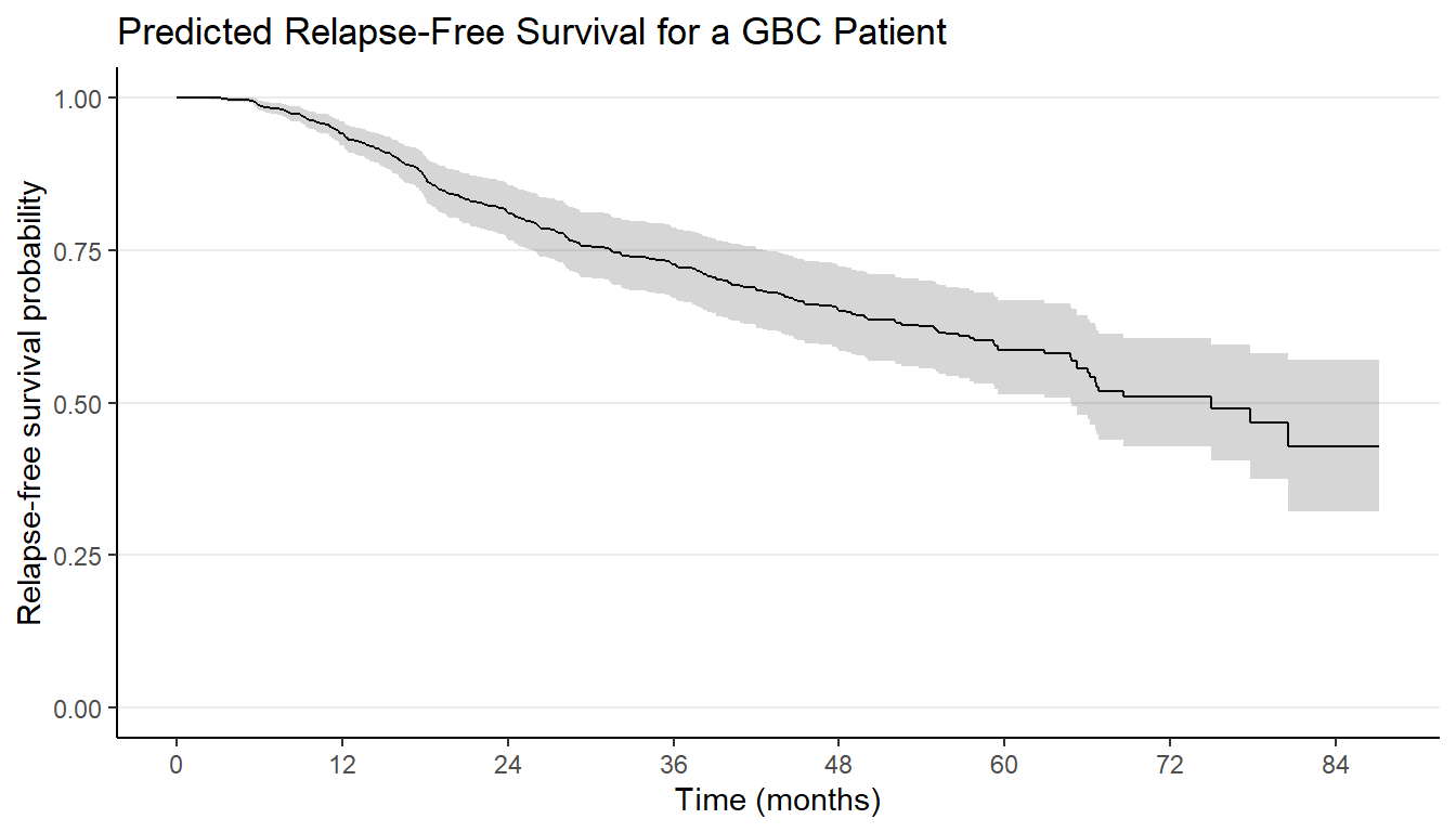
Prediction Graphics Exercise

Task: Add horizontal grid lines

Solution

pred_fig + theme(panel.grid.major.y = element_line()) # Add horizontal grid lines

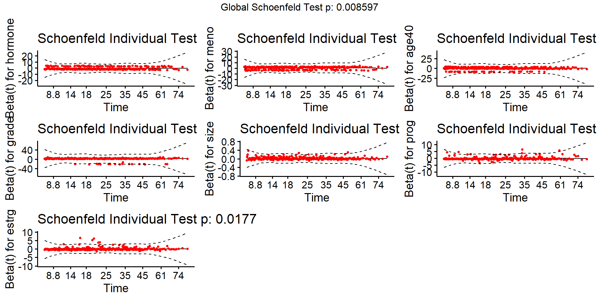
Cox Model Diagnostics

PH assumptions: Schoenfeld residuals
- Difference between observed and expected covariate values at each event time
- Use cox.zph() to test PH assumption
- Use survminer::ggcoxzph() on cox.zph object to visualize Schoenfeld residuals
Functional form of covariates
- Plot martingale residuals against (quantitative) covariates
- Use residuals(cox_fit, type = "martingale") to get martingale residuals
Other aspects
- Appropriateness of exponential link function
- Influential points/outliers
- survminer::ggcoxdiagnostics()

Schoenfeld Residuals

Check proportionality

Focus on graphics; use \(p\)-value only as guideline

library(survminer) # Load survminer package
ph_test <- cox.zph(cox_fit) # Test proportional hazards assumption
ggcoxzph(ph_test) # Visualize Schoenfeld residuals

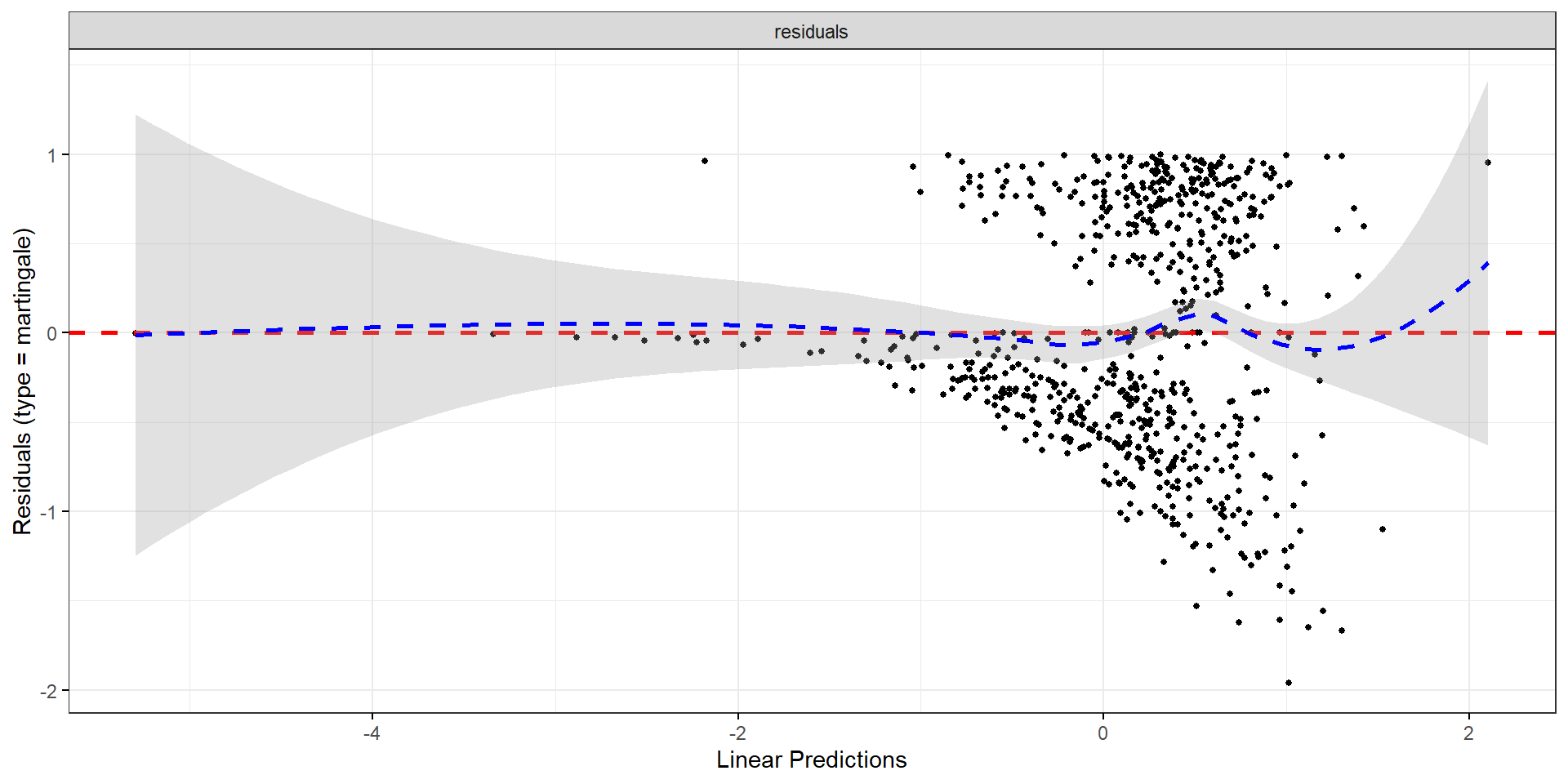
Exponential Link Function

Martingale vs. \(\hat\beta^\mathrm{T} Z_i\)

# Martingale residuals vs linear predictor
ggcoxdiagnostics(cox_fit, type = "martingale",    # martingale on y-axi
                 ox.scale = "linear.predictions") # linear predictor on x-axis

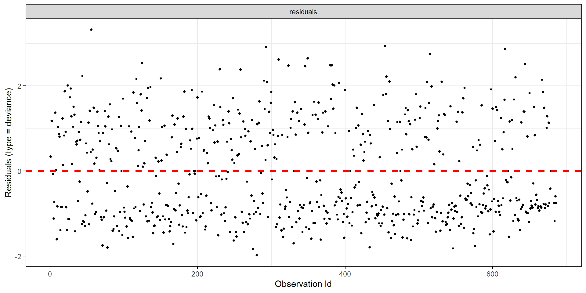
Influential Points

Deviance residuals

# Deviance residuals vs linear predictor
ggcoxdiagnostics(cox_fit, type = "deviance",  # deviance on y-axis
                 ox.scale = "observation.id", # observation ID on x-axis
                 sline = FALSE)               # no smoothed line

General Residual Graphics

Basic arguments of ggcoxdiagnostics()
- coxph object
- type: Residual type (“martingale”, “deviance”, “score”, “schoenfeld”, “dfbeta”, “dfbetas”, and “scaledsch”)`
- ox.scale: Scale for x-axis (“linear.predictions”, “observation.id”, “time”)
- point.col: Color of points
- point.size: Size of points
- etc.
More about survminer
- survminer website

Competing Risks Regression

Sub-Distribution Hazard

Definition \[ \Lambda_k(t\mid Z) = -\log\left\{1 - F_k(t\mid Z)\right\} \]
- \(F_k(t \mid Z)\): cumulative incidence function (CIF) of the \(k\)-th cause
- \(\lambda_k(t \mid Z)=\Lambda_k'(t\mid Z)\): risk of the \(k\)-th cause in presence of other competing events in the whole population
Different from cause-specific hazard
- Cause-specific hazard \[\lambda^\mathrm{c}_k(t \mid Z) = \Pr(t\leq T< t+ \mathrm{d}t, \Delta = k\mid T\geq t, Z)/\mathrm{d}t \]
- Risk of the \(k\)-th cause in survivors

Fine-Gray Model

Proportional sub-distribution hazards \[ \lambda_k(t \mid Z) = \lambda_0(t) \exp(\beta_1 Z_1 + \beta_2 Z_2 + \ldots + \beta_p Z_p)\]
- \(\lambda_0(t)\): baseline sub-distribution hazard function
- \(\exp(\beta_j)\): sub-distribution hazard ratio for covariate \(Z_j\)

library(tidycmprsk) # Load tidycmprsk package
data("trial", package = "tidycmprsk") # Load trial data from tidycmprsk package
head(trial) # Display the first few rows of the data

# A tibble: 6 × 9
  trt      age marker stage grade response death death_cr           ttdeath
  <chr>  <dbl>  <dbl> <fct> <fct>    <int> <int> <fct>                <dbl>
1 Drug A    23  0.16  T1    II           0     0 censor                24  
2 Drug B     9  1.11  T2    I            1     0 censor                24  
3 Drug A    31  0.277 T1    II           0     0 censor                24  
4 Drug A    NA  2.07  T3    III          1     1 death other causes    17.6
5 Drug A    51  2.77  T4    III          1     1 death other causes    16.4
6 Drug B    39  0.613 T4    I            0     1 death from cancer     15.6

Fitting Fine-Gray Model

Using cmprsk::crr()
- formula: Surv(time, status) ~ covariates
  - status: a factor with first level indicating censoring and subsequent levels the competing risks
- failcode: event code for the cause of interest

fg_fit <- crr(Surv(ttdeath, death_cr) ~ trt + age + marker + stage, # fit FG model
              failcode = "death from cancer", trial) # for death from cancer

21 cases omitted due to missing values

fg_fit # print the Fine-Gray model fit summary


Variable    Coef     SE      HR     95% CI       p-value    
trtDrug B   0.396    0.283   1.49   0.85, 2.59   0.16       
age         0.009    0.011   1.01   0.99, 1.03   0.42       
marker      -0.002   0.159   1.00   0.73, 1.36   0.99       
stageT2     0.140    0.475   1.15   0.45, 2.92   0.77       
stageT3     0.500    0.460   1.65   0.67, 4.06   0.28       
stageT4     0.959    0.418   2.61   1.15, 5.91   0.022

Parameter Estimates and Variance

Extracting \(\hat\beta\) and \(\hat{\mathrm{var}}(\hat\beta)\)

coef(fg_fit) # Extract coefficients

   trtDrug B          age       marker      stageT2      stageT3      stageT4 
 0.396486121  0.008956935 -0.002006717  0.140251967  0.500394141  0.958640247

vcov(fg_fit) |> head() # Extract variance-covariance matrix

              [,1]          [,2]          [,3]         [,4]          [,5]
[1,]  0.0800665101  0.0001535045 -0.0051801922  0.011605373  0.0094601803
[2,]  0.0001535045  0.0001239790 -0.0005094795  0.001111245 -0.0009368412
[3,] -0.0051801922 -0.0005094795  0.0251827414 -0.028697647 -0.0037297926
[4,]  0.0116053732  0.0011112447 -0.0286976466  0.225187822  0.1101888313
[5,]  0.0094601803 -0.0009368412 -0.0037297926  0.110188831  0.2111942725
[6,]  0.0219362509  0.0010459739 -0.0176113331  0.124589145  0.1064088264
             [,6]
[1,]  0.021936251
[2,]  0.001045974
[3,] -0.017611333
[4,]  0.124589145
[5,]  0.106408826
[6,]  0.174446817

Tidy Fine-Gray Model Output

Using broom package: broom::tidy()
- Provides a tidy data frame for easy manipulation and visualization

tidy_fg <- tidy(fg_fit, exponentiate = TRUE, conf.int = TRUE) # Tidy model output
tidy_fg # Display the tidy output

# A tibble: 6 × 7
  term      estimate std.error statistic conf.low conf.high p.value
  <chr>        <dbl>     <dbl>     <dbl>    <dbl>     <dbl>   <dbl>
1 trtDrug B    1.49     0.283     1.40      0.854      2.59   0.16 
2 age          1.01     0.0111    0.804     0.987      1.03   0.42 
3 marker       0.998    0.159    -0.0126    0.731      1.36   0.99 
4 stageT2      1.15     0.475     0.296     0.454      2.92   0.77 
5 stageT3      1.65     0.460     1.09      0.670      4.06   0.28 
6 stageT4      2.61     0.418     2.30      1.15       5.91   0.022

Forest Plot Exercise

Task: Visualize sub-distribution hazard ratios and confidence intervals

Solution

# tidy_fg$term <- recode(tidy_fg$term, ...) # Relabel the variables
tidy_fg |>  # plot of sub-distribution hazard ratios and 95% CIs
  ggplot(aes(y=term, x=estimate, xmin=conf.low, xmax=conf.high)) + 
  geom_pointrange() +  # plots center point (x) and range (xmin, xmax)
  geom_vline(xintercept=1, linetype = 2) + # vertical line at HR=1
  scale_x_log10("Sub-distribution hazard ratio (95% CI)") + # log scale for x-axis
  theme_classic() + # classic theme for clean look
  theme(
    axis.line.y = element_blank(),          # remove y-axis line
    axis.ticks.y = element_blank(),         # remove y-axis ticks
    axis.text.y = element_text(size = 11),  # set variable label size
    axis.title.y = element_blank()          # remove y-axis title
  )

FG Regression Table (I)

Using gtsummary package: tbl_regression()
- Similarly to tabulating fitted coxph object

library(gtsummary) # Load gtsummary package
fg_tbl <- fg_fit |> tbl_regression(exponentiate = TRUE) |>  # Create a regression table 
          add_global_p() # Add global p-value for categorical variables

FG Regression Table (II)

Result

Characteristic	HR¹	95% CI¹	p-value
Chemotherapy Treatment			0.2
Drug A	—	—
Drug B	1.49	0.85, 2.59
Age	1.01	0.99, 1.03	0.4
Marker Level (ng/mL)	1.00	0.73, 1.36	>0.9
T Stage			0.058
T1	—	—
T2	1.15	0.45, 2.92
T3	1.65	0.67, 4.06
T4	2.61	1.15, 5.91
¹ HR = Hazard Ratio, CI = Confidence Interval

Model-Based Prediction

Predicted cumulative incidence function (CIF) \[ \hat F_k(t \mid z) = 1 - \exp\left\{-\hat\Lambda_k(t \mid z)\right\} \]

# Predict cumulative incidence function for first 10 patients
fg_pred <- predict(fg_fit, newdata= trial[1:10, ], times = c(6, 12, 18)) # Predict CIF
fg_pred # Display the predicted CIF

$`time 6`
 [1] 0.002279375 0.003430702 0.002447917          NA 0.007579470 0.010150002
 [7] 0.002582498 0.002462688 0.002448570 0.006155050

$`time 12`
 [1] 0.02093164 0.03135502 0.02246374         NA 0.06809922 0.09023665
 [7] 0.02368558 0.02259790 0.02246967 0.05562630

$`time 18`
 [1] 0.07090010 0.10483563 0.07594466         NA 0.21744137 0.28018810
 [7] 0.07995368 0.07638548 0.07596414 0.18042196

Summary

Key Takeaways

Cox proportional hazards regression
- Tidy output with broom and gtsummary
- Visualize hazard ratios with forest plots with ggplot2
- Model-based prediction with survival::survfit() and ggsurvfit()
- Model diagnostics with survminer
Fine-Gray model for competing risks regression
- Fit with cmprsk::crr()
- Tidy output with broom and gtsummary
- Visualize sub-distribution hazard ratios with forest plots

Next Steps

Machine learning: build best predictive model with many predictors
- Regularized Cox regression
- Parametric AFT models
- Survival trees
- tidymodels packages (censored)

Tidy Survival Analysis: Applying R’s Tidyverse to Survival Data

Presenting Regression Results

Cox PH Regression

GBC Data: a Running Example

Analysis in Base R

Tidy coxph() Output

Tabulating Results with gtsummary (I)

Tabulating Results with gtsummary (II)

Further Customization

Table Customization Exercise

Other Regression Models

Visualizing Hazard Ratios (I)

Visualizing Hazard Ratios (II)

Forest Plot Exercise

Cox Model Prediction and Diagnostics

Model-Based Prediction

Tidy Survival Prediction

Visualizing Predicted Survival (I)

Visualizing Predicted Survival (II)

Prediction Graphics Exercise

Cox Model Diagnostics

Schoenfeld Residuals

Exponential Link Function

Influential Points

General Residual Graphics

Competing Risks Regression

Sub-Distribution Hazard

Fine-Gray Model

Fitting Fine-Gray Model

Parameter Estimates and Variance

Tidy Fine-Gray Model Output

Forest Plot Exercise

FG Regression Table (I)

FG Regression Table (II)

Model-Based Prediction

Summary

Key Takeaways

Next Steps

Tidy `coxph()` Output

Tabulating Results with `gtsummary` (I)

Tabulating Results with `gtsummary` (II)