Tidy Survival Analysis: Applying R’s Tidyverse to Survival Data
Module 2. Data Manipulation with Tidyverse
Lu Mao
Department of Biostatistics & Medical Informatics
University of Wisconsin-Madison
Aug 3, 2025
Overview of Tidyverse
The tidyverse Ecosystem
Motivation: tidy data for reproducible analysis
Key packages
dplyr(filtering, mutating, grouping, summarizing)tidyr(pivoting, nesting, reshaping)tibble(modern data frames)readr/haven(importing .csv or .sas7bdat)lubridate(handling time variables)ggplot2(visualization)
Basic Functionalities
- Data manipulation: using
dplyrverbsmutate()to create new variables (e.g., age group, log-transformed labs)filter()to subset by treatment or ageselect()andrename()for variable formattingarrange()to sortgroup_by()andsummarize()for descriptive summaries by arm
- Data reshaping: using
tidyrfunctionspivot_longer()to convert wide to long formatpivot_wider()to convert long to wide formatnest()andunnest()for hierarchical data
A Simple Example
- Example dataset
# Simulated data example
df1 <- tibble(
  id = 1:6,
  trt = c("A", "A", "B", "B", "A", "B"),
  age = c(65, 70, 58, 60, 64, 59),
  time = c(5, 8, 12, 3, 2, 6),
  status = c(1, 0, 1, 1, 0, 0)  # 1 = event, 0 = censored
)
df1
# A tibble: 6 × 5
id trt age time status
<int> <chr> <dbl> <dbl> <dbl>
1 1 A 65 5 1
2 2 A 70 8 0
3 3 B 58 12 1
4 4 B 60 3 1
5 5 A 64 2 0
6 6 B 59 6 0Native Pipe Operator: |>
- What is
|>- Introduced in R 4.1 (hot key:
Ctrl + Shift + M) - Passes the result of one expression into the first argument of the next
- Same idea as
%>%, but built into base R
- Introduced in R 4.1 (hot key:
- Example
df1 |> # passes tibble data frame df1 to the next function
  mutate(age_group = if_else(age >= 65, "older", "younger")) |> # create age group
  filter(trt == "A") |> # filter for treatment A
  arrange(time) # sort by time
# A tibble: 3 × 6
id trt age time status age_group
<int> <chr> <dbl> <dbl> <dbl> <chr>
1 5 A 64 2 0 younger
2 1 A 65 5 1 older
3 2 A 70 8 0 older Summarizing and Grouping
Survival-specific summaries (e.g., number of events)
group_by()andsummarize()for descriptive summaries by arm
df1 |>
  group_by(trt) |> # group by treatment arm
  summarize( # summarize each group
    n = n(), # count number of rows (subjects)
    events = sum(status), # sum of events (status = 1)
    median_time = median(time) # median survival time
  )
# A tibble: 2 × 4 trt n events median_time <chr> <int> <dbl> <dbl> 1 A 3 1 5 2 B 3 2 6
What Does “Tidy” Mean?
A dataset is tidy if:
- Each variable is a column
- Each observation is a row
- Each type of observational unit is a table
— Hadley Wickham, Tidy Data (2014)
https://www.jstatsoft.org/article/view/v059i10
Why Tidy Data?
- Tidy data principles
- Easy to reshape and transform
- Compatible with
ggplot2,dplyr,tidyr, and modeling tools - Encourages modular and reproducible code
- Messy data challenges
- Time in rows, covariates in columns
- Multiple data types in one column
- Separate randomization and event/censoring dates
- Missing/censored values inconsistently coded
Tidy Survival Data
- Possible pre-processing steps
- Calculate survival time from start to event/censoring
- Creating the \((X, \delta)\) structure expected by
Surv() - Reshaping data to long format in case of multiple events
- An Example
  id     time status hormone age meno size grade nodes prog estrg
1  1 43.83607      1       1  38    1   18     3     5  141   105
2  1 74.81967      0       1  38    1   18     3     5  141   105
3  2 46.55738      1       1  52    1   20     1     1   78    14
4  2 65.77049      0       1  52    1   20     1     1   78    14
5  3 41.93443      1       1  47    1   30     2     1  422    89
6  3 47.73770      2       1  47    1   30     2     1  422    89
Tidying Survival Data
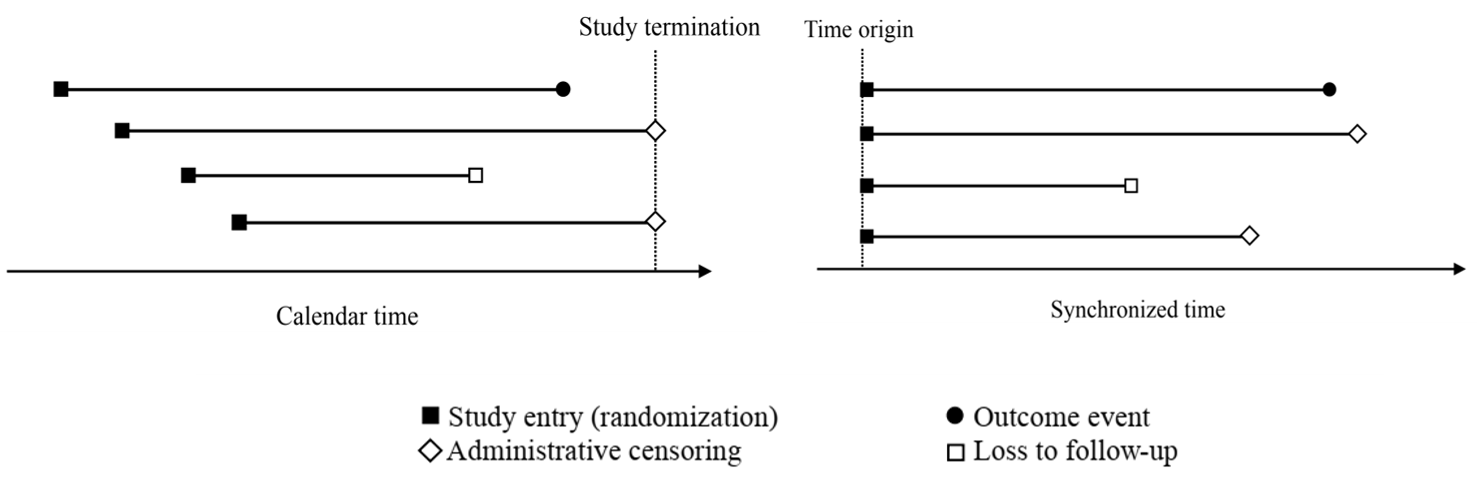
Calendar vs. Event Times
- Time from start to event/censoring (\(X\))
Dates to Time Difference
- A data example
# Example: raw dates as character strings
df2 <- tibble(
  id = 1:3,
  rand_date = c("2022-01-01", "2022-01-15", "2022-01-20"),
  end_date = c("2022-04-01", "2022-06-01", "2022-03-15"),
  status = c("dead", "censored", "dead")
)
df2
# A tibble: 3 × 4
id rand_date end_date status
<int> <chr> <chr> <chr>
1 1 2022-01-01 2022-04-01 dead
2 2 2022-01-15 2022-06-01 censored
3 3 2022-01-20 2022-03-15 dead Parsing Dates and Calculating Time
Using
lubridateto parse datesymd()for “year-month-day” formatmdy()for “month-day-year” format
# Parse dates and calculate time/status
df2 |>
  mutate(
    rand_date = ymd(rand_date), # convert character to Date
    end_date = ymd(end_date), # convert character to Date
    time = as.numeric(end_date - rand_date), # calculate time in days
    status = if_else(status == "dead", 1, 0) # convert status to 1/0
  )
# A tibble: 3 × 5 id rand_date end_date status time <int> <date> <date> <dbl> <dbl> 1 1 2022-01-01 2022-04-01 1 90 2 2 2022-01-15 2022-06-01 0 137 3 3 2022-01-20 2022-03-15 1 54
Exercise: Calculate Survival Time (I)
- Calculate
timeandstatusvariables fordf3:
# create a df3 with dates in the form of month-day-year
df3 <- tibble(
  id = 1:3,
  rand_date = c("Jan-01-2022", "01-15-2022", "01-20-2022"),
  end_date = c("04-01-2022", "Jun-01-2022", "03-15-2022"),
  status = c("dead", "censored", "dead")
)
df3
# A tibble: 3 × 4
id rand_date end_date status
<int> <chr> <chr> <chr>
1 1 Jan-01-2022 04-01-2022 dead
2 2 01-15-2022 Jun-01-2022 censored
3 3 01-20-2022 03-15-2022 dead Exercise: Calculate Survival Time (II)
- Hint: use
mdy()to parse dates
- More about manipulating dates
- lubridate official documentation
- R for Data Science: Dates and times
Parsing Censored Observations
Alternative formats for censored times
"32+",">17", etcparse_number()for gettime;str_detect()forstatus
# Example data: relapse times with "+" indicating censoring
MP <- c(10,  "32+", 23, "25+")
# Convert to (time, status) format
df4 <- tibble(
  MP = MP,                               # Original data
  time = parse_number(MP),               # Extract numeric part
  status = 1 - str_detect(MP, "\\+")     # Censored if "+" detected
)
df4
# A tibble: 4 × 3 MP time status <chr> <dbl> <dbl> 1 10 10 1 2 32+ 32 0 3 23 23 1 4 25+ 25 0
Exercise: Parse Censored Times
- Task: Parse
MPindf5to createtimeandstatus
Reshaping Data
- Why reshape?
- Multiple events per subject
- Wide format (multiple columns) \(\rightarrow\) long format (one row per event)
# Example: wide format with multiple events
df6 <- tibble(
  id = 1:3,
  prog_time = c(10, 20, 30),
  prog_status = c(1, 0, 1), # 1 = progression, 0 = censored
  death_time = c(15, 20, 35),
  death_status = c(0, 1, 1) # 1 = dead, 0 = censored
)
df6
# A tibble: 3 × 5
id prog_time prog_status death_time death_status
<int> <dbl> <dbl> <dbl> <dbl>
1 1 10 1 15 0
2 2 20 0 20 1
3 3 30 1 35 1Wide to Long
- Using
pivot_longer()- Convert wide format to long format
- Specify
names_toandvalues_tofor new columns
df7 <- df6 |>
  pivot_longer(
    cols = c(prog_time, prog_status, death_time, death_status), # columns to reshape
    names_to = c("event", ".value"), # .value keeps the variable name, event is the new column
    names_pattern = "(.*)_(.*)" # split by underscore
  )
df7
# A tibble: 6 × 4
id event time status
<int> <chr> <dbl> <dbl>
1 1 prog 10 1
2 1 death 15 0
3 2 prog 20 0
4 2 death 20 1
5 3 prog 30 1
6 3 death 35 1Exercise: Clean Up
- Task: Clean up
df7to create a tidy survival dataset- Remove rows with
event = progandstatus = 0(non-terminal event) - Recode
status = 2for death events
- Remove rows with
Solution
df7 |>
  filter(
    !(event == "prog" & status == 0) # remove non-occurrence of non-terminal events
    ) |>
  mutate(
    status = if_else(event == "death" & status == 1, 2, status) # recode death status
  )
# # A tibble: 5 × 4
#      id event  time status
#   <int> <chr> <dbl>  <dbl>
# 1     1 prog     10      1
# 2     1 death    15      0
# 3     2 death    20      2
# 4     3 prog     30      1
# 5 3 death 35 2- More on reshaping data
- tidyr official documentation
- R for Data Science: Data tidying
Visualizing Subject Follow-Up
Swimmer Plot
- What is a swimmer plot?
- Visualizes subject follow-up
- Each row represents a subject
- Horizontal lines show time to event/censoring
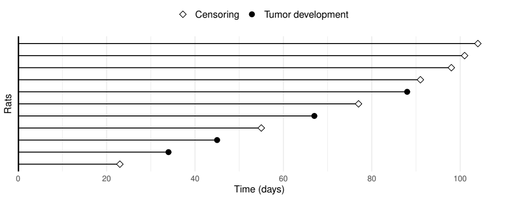
Swimmer Plot Basics
- Using
ggplot2geom_linerange()for horizontal linesgeom_point()for eventsfacet_wrap()for treatment arms (optional)
- A data example
# Example data: rat survival times
df8 <- tibble(
  time = c(101, 55, 67, 23, 45, 98, 34, 77, 91, 104, 88),
  status = c(0, 0, 1, 0, 1, 0, 1, 0, 0, 0, 1),
  group = c("A", "A", "A", "B", "B", "B", "A", "B", "B", "A", "B")
) |>
  mutate(
    id = row_number(), # create id column using row number
    .before = 1 # place id before time
  )
Creating a Swimmer Plot
- Code to reproduce previous plot
# Specify the plot
fig8 <- df8 |>
  # Set-up: id on the y-axis, time on the x-axis
  ggplot(aes(x = time, y = reorder(id, time))) + # reorder id by time
  # Add geometric objects
  geom_linerange(aes(xmin = 0, xmax = time)) + # horizontal lines from 0 to time
  # Add points for events/censoring, distinguish by status
  geom_point(aes(shape = factor(status)), size = 2.5, fill = "white") +
  # Add vertical line at x = 0
  geom_vline(xintercept = 0, linewidth = 1) +
  theme_minimal() + # use minimal theme
  # Format y axis
  scale_y_discrete(name = "Rats") + # y-axis label
  # Format x axis (label, breaks, no expansion on left, 0.05 expansion on right)
  scale_x_continuous(name = "Time (days)", breaks = seq(0, 100, by = 20),
                     expand = expansion(c(0, 0.05))) +
  # Format point shape (pch = 23 for censoring, pch = 19 for event; label shape)
  scale_shape_manual(values = c(23, 19), labels = c("Censoring", "Tumor development")) +
  # Further formatting using theme()
  theme(
    legend.position = "top", # place legend at the top
    legend.title = element_blank(), # no legend title
    axis.text.y = element_blank(), # no y-axis labels (otherwise id's will be printed)
    axis.ticks.y = element_blank(), # no y-axis ticks
    panel.grid.major.y = element_blank(), # no major grid lines on y-axis
    legend.text = element_text(size = 11) # legend text size
  )

# Display the plot
fig8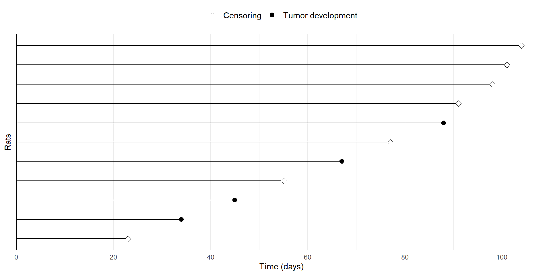
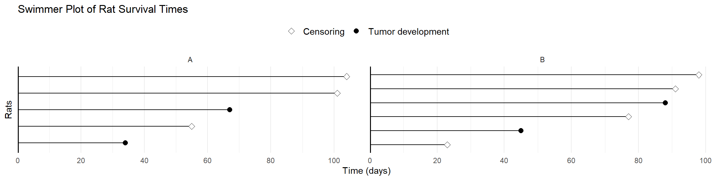
Exercise: Swimmer Plot by Group
- Task: Create a swimmer plot for
df8bygroup- Use
facet_wrap()to create separate panels for each group - Add a title “Swimmer Plot of Rat Survival Times”
- Use
Creating “Table 1”
Descriptive Statistics
- Importance of Table 1
- Summarizes baseline characteristics
- Provides context for formal analysis
- Using
gtsummarytbl_summary()for descriptive statisticsadd_p()for p-values comparing groups (not recommended for randomized trials)add_overallto add overall summarymodify_header()to customize table headers
Basic Syntax of tbl_summary()
- Common arguments
by = "group"to summarize by groupinclude = c("variable1", "variable2")to include specific variableslabel = list(variable = "Label")to customize variable labelsstatistic = list(variable ~ "statistic")to specify statisticsstatistic = list(all_continuous() ~ "{mean} ({sd})")for mean and SD
digits = list(variable ~ 2)to set decimal places
A Simple Example
- Example dataset
# Example data: 10 subjects with treatment, age, and sex
df9 <- tibble(
  id = 1:10,
  time = c(101, 55, 67, 23, 45, 98, 34, 77, 91, 104),
  status = c(0, 1, 1, 0, 1, 0, 1, 0, 1, 0), # 0 = censored, 1 = event
  trt = c("A", "A", "B", "B", "A", "B", "A", "B", "A", "B"),
  sex = c("M", "F", "M", "F", "M", "F", "M", "F", "M", "F"),
  age = c(65, 70, 58, 60, 64, 59, 66, 62, 68, 61)
)
head(df9)
# A tibble: 6 × 6
id time status trt sex age
<int> <dbl> <dbl> <chr> <chr> <dbl>
1 1 101 0 A M 65
2 2 55 1 A F 70
3 3 67 1 B M 58
4 4 23 0 B F 60
5 5 45 1 A M 64
6 6 98 0 B F 59Creating a Summary Table
library(gtsummary) # load package
df9 |>
  tbl_summary(
    by = trt,                            # summarize by treatment arm
    include = c(sex, age, time, status), # include specific variables
    label = list(                        # label variables
      time = "Follow-up time (months)",
      status = "Events"
    )
)| Characteristic | A, N = 51 | B, N = 51 |
|---|---|---|
| sex | ||
| F | 1 (20%) | 4 (80%) |
| M | 4 (80%) | 1 (20%) |
| age | 66.0 (65.0, 68.0) | 60.0 (59.0, 61.0) |
| Follow-up time (months) | 55 (45, 91) | 77 (67, 98) |
| Events | 4 (80%) | 1 (20%) |
| 1 n (%); Median (IQR) | ||
Exercise: Summarize GBC Data (I)
- Task: Summarize the GBC mortality data (
gbc_mort.txt) like below
| Characteristic | Hormone, N = 2461 | No Hormone, N = 4401 | Overall, N = 6861 |
|---|---|---|---|
| Follow-up time (months) | 48 (29, 61) | 41 (25, 57) | 44 (26, 60) |
| Death | 56 (23%) | 115 (26%) | 171 (25%) |
| Age (years) | 58 (50, 63) | 50 (45, 59) | 53 (46, 61) |
| Menopausal status | 187 (76%) | 209 (48%) | 396 (58%) |
| Tumor size (mm) | 25 (20, 35) | 25 (20, 35) | 25 (20, 35) |
| Tumor grade | |||
| 1 | 33 (13%) | 48 (11%) | 81 (12%) |
| 2 | 163 (66%) | 281 (64%) | 444 (65%) |
| 3 | 50 (20%) | 111 (25%) | 161 (23%) |
| Number of nodes | 3 (1, 7) | 3 (1, 7) | 3 (1, 7) |
| Progesterone (fmol/mg) | 35 (7, 133) | 32 (7, 130) | 33 (7, 132) |
| Estrogen (fmol/mg) | 46 (9, 183) | 32 (8, 92) | 36 (8, 114) |
| 1 Median (IQR); n (%) | |||
Exercise: Summarize GBC Data (II)
- Points to note
- Summarize by hormone therapy (
hormone) - Include variables:
time,status,age,meno,size,grade,nodes,prog,estrg - Label variables appropriately
- Add overall summary column at the end
- Summarize by hormone therapy (
Exercise: Summarize GBC Data (III)
Solution
# Load GBC mortality data (one record per patient)
gbc_mort <- read.table("data/gbc_mort.txt")
# Create the summary table
gbc_mort |>
  mutate( # relabel hormone and menopausal status
    hormone = if_else(hormone == 1, "No Hormone", "Hormone"),
    meno = if_else(meno == 1, "No", "Yes")
  ) |>
  tbl_summary( # create table
    by = hormone, # summarize by hormone therapy
    include = ! id, # exclude id from summary
    # Label variables
    label = list(
      time = "Follow-up time (months)",
      status = "Death",
      hormone = "Hormone therapy",
      age = "Age (years)",
      meno = "Menopausal status",
      size = "Tumor size (mm)",
      grade = "Tumor grade",
      nodes = "Number of nodes",
      prog = "Progesterone (fmol/mg)",
      estrg = "Estrogen (fmol/mg)"
    ),
  ) |>
  add_overall(last = TRUE) # Add overall column, at the end
Exercise: Summarize GBC Data (IV)
- Task: summarize relapse and death data from
gbc.txt- Hint:
group_by(id)andsummarize()
- Hint:
| Characteristic | Hormone, N = 2461 | No Hormone, N = 4401 | Overall, N = 6861 |
|---|---|---|---|
| Relapse | 94 (38%) | 205 (47%) | 299 (44%) |
| Death | 56 (23%) | 115 (26%) | 171 (25%) |
| Composite | 94 (38%) | 205 (47%) | 299 (44%) |
| Relapse then death | 56 (23%) | 115 (26%) | 171 (25%) |
| 1 n (%) | |||
Exercise: Summarize GBC Data (V)
Solution
# Load GBC relapse and death data (long format)
gbc <- read.table("data/gbc.txt")
# Create the summary table
gbc |>
  group_by(id, hormone) |>
  summarize(
    rel = any(status == 1), # boolean for existence of a relapse (status=1)
    death = any(status == 2), # boolean for existence of a death (status=2)
    comp = rel | death,  # boolean for existence of either relapse or death
    both = rel & death, # boolean for existence of both relapse and death
  ) |>
  mutate(
    hormone = if_else(hormone == 1, "No Hormone", "Hormone") # relabel hormone therapy
  ) |>
  tbl_summary( # create table
    by = hormone, # summarize by hormone therapy
    include = c(rel, death, comp, both), # include specific variables
    # Label variables
    label = list(
      rel = "Relapse",
      death = "Death",
      comp = "Composite",
      both = "Relapse then death"
    )
  ) |>
  add_overall(last = TRUE) # Add overall column, at the end
Summary
Key Takeaways
- Tidyverse provides powerful tools for data manipulation and visualization
- Tidy data principles simplify analysis and visualization
- Survival data may require pre-processing steps (
dplyr,tidyr,lubridate) - Swimmer plots effectively visualize subject follow-up (
ggplot2) - Descriptive statistics can be easily summarized using
gtsummary::tbl_summary()
Next Steps
- Format analysis results from the
survivalpackage:- Nonparametric estimates with
survfit() - Regression models with
coxph()
- Nonparametric estimates with
- Explore advanced visualization techniques:
- Kaplan–Meier curves with
ggsurvfitorsurvminer - Layered plots using
ggplot2 - Annotated plots for publications
- Kaplan–Meier curves with