library(survival)
source("DORfunctions.R")Analysis of duration of response in oncology studies
This R-code implements the analysis of duration-of-response data described in Mao et al. (2024) for oncology studies .
Background
Duration-of-response (DOR) is often utilized to assess efficacy of oncology therapies. While valid procedures are available for estimating the mean of DOR (Huang et al. 2018, 2020; Huang and Tian 2022), it is unclear how to estimate its distribution, which may provide a fuller picture. Simple Kaplan–Meier estimates based on the responders can result in distorted conclusions as they ignore the existence of non-responders (whose DOR is zero).
Notation and Methodology
Full and Observed Data
For a responder, let T_1 denote the time to response. Let T_2 denote the time to disease progression or death. If a patient experiences progression/death first, then T_1=\infty. The DOR can be defined as [T_2-T_1]_+, where x_+=xI(x>0). Thus, DOR is T_2-T_1 for responders, i.e., those with T_1<\infty, and 0 for nonresponders. For notational convenience, set T_1=T_2 for nonresponders.
Due to limited follow-up, the entire distribution of DOR is not identifiable. Instead, we define the restricted DOR within a time window as D=T_2\wedge \tau -T_1\wedge \tau, where \tau is a pre-specified restriction time. Our goal is to estimate the survival function of D: S_D(t)=P(D>t), \,\,\,\,\, t\in [0, \tau].
Let C denote the censoring time independent of (T_1, T_2) and satisfying P(C\geq \tau)>0. Then we observe (X_1,\Delta_1,X_2,\Delta_2), where X_1=\min(T_1\wedge\tau, C), \Delta_1=I(T_1\wedge\tau\leq C), X_2=\min(T_2\wedge\tau,C), and \Delta_2=I(T_2\wedge\tau\leq C). Write \tilde D=X_2 - X_1. Here both T_1 and T_2 are subject to the same censoring time C. The observed data consist of n independent and identically distributed (i.i.d.) copies of (X_1,\Delta_1,X_2,\Delta_2): \{\mathcal O_i\equiv (X_{1i},\Delta_{1i},X_{2i},\Delta_{2i}): i=1,\ldots,n\}. Write \tilde D_i=X_{2i}- X_{1i}.
Estimation and Inference
A simple estimator of S_D(t) is the inverse probability censoring weighted (IPCW) estimator: \hat S_D(t)=n^{-1}\sum_{i=1}^n \frac{\Delta_{2i}}{\hat{G}_C(X_{2i})} I(\tilde D_i> t), where \hat{G}_C(t) is the Kaplan–Meier estimator of G_C(t)=P(C>t) based on \{(X_{2i}, 1-\Delta_{2i}), i=1, \cdots, n\}. To see \hat S_D(t) as a valid estimator, note that \Delta_{2}=1 implies that X_2=T_2\wedge\tau, X_1=T_1\wedge\tau and thus that \tilde D = D. Hence, E\left\{\Delta_2I(\tilde D>t)/G_C(X_2)\right\}= E\left\{\Delta_2I(D>t)/G_C(T_2\wedge\tau)\right\} =E\left[E\left\{\Delta_2I(D>t)/G_C(T_2\wedge\tau)\mid T_1, T_2\right\}\right] =E\{I(D>t)\}=S_D(t), where the second equality follows by the independence of C and (T_1, T_2). Moreover, we can show that \hat S_D(t) converges weakly to a Gaussian process with an easily estimable variance function.
The median DOR can thus be estimated by \inf\{t: \hat S_D(t)\leq 0.5\}, whose variance can be estimated by perturbing the influence functions of \hat S_D(t) with standard normal random noises. Details about the inference on \hat S_D(t) and the median can be found in Appendix.
Usage and Example
R-program
To use the program, download DORfunctions.R from repo https://github.com/lmaowisc/dor. The R-file contains all functions needed to perform the analysis. We also need the standard survival package.
The main function is dorfit(x1, delta1, x2, delta2, tau, med_inf = FALSE).
Input
x1time to earliest of response, outcome event, or censoring (X_1)delta1indicator of response (\Delta_1)x2time to earlier of outcome event and censoring (X_2)delta2indicator of outcome event (\Delta_2)taurestriction time (\tau)med_infwhether to make inference on the median DOR (default isFALSE)
Output
t1vector of times (t)surv1IPCW estimates of survival function \hat S_D(t)se1pointwise standard error of \hat S_D(t)medmedian estimate of DORmed_se, med_lo, med_hithese are standard error, lower and upper limits of the 95% confidence interval of the median, respectively, ifmed_inf = TRUE; allNULLifmed_inf = FALSE
A simulated example
Let’s simulate a data set of size n=200.
# set seed for random number generation
set.seed(2023)

## simulate data
n <- 200
# set restriction time
tau <- 1.25

# full data
t1 <- pmin(rexp(n), runif(n, 0, 0.75)) # response time
t2 <- rexp(n)*1.5 # outcome event time
t1[t1>t2] <- t2[t1>t2] # set t1 = t2 for non-responders
c <- runif(n, 0, 1.5) # censoring time

# observed (censored) data
x1 <- pmin(t1, c)
delta1 <- 1*(t1<c)
x2 <- pmin(t2, c)
delta2 <- 1*(t2<c)
So the observed data consist of x1, delta1, x2, and delta2. Under restriction time tau= 1.25. We analyze the DOR distribution using the main function dorfit(), with inference on the median.
fitLM <- dorfit(x1, delta1, x2, delta2, tau, med_inf = TRUE)Let’s plot the estimated S_D(t) with 95% pointwise confidence limits.
za <- qnorm(0.975)
## marginal survival function P(D > t)
t <- fitLM$t1 # times
St <- fitLM$surv1 # P(D > t)
se <- fitLM$se1 # se of P(D > t)

# set up the figure
plot(c(0, 1.2), c(0, 1), type="n",xlab="t",ylab=expression(S[D](t)))

# plot the marginal curve P(D > t)
lines(stepfun(t, c(1,St)),lwd=2, do.points = FALSE) # marginal
lines(stepfun(t, c(1,St + za * se)),lty = 3, do.points = FALSE) # upper 95% CI
lines(stepfun(t, c(1,St - za * se)),lty = 3, do.points = FALSE) # lower 95% CI 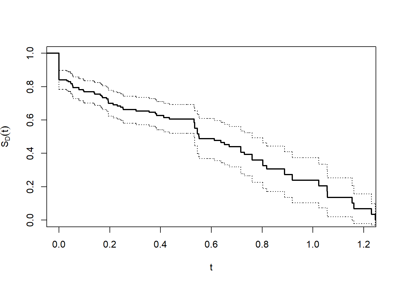
We can see that the median is close to 0.6. The precise number and confidence interval (CI) can be obtained from fitLM.
######## get the median ####
med <- fitLM$med
med
# [1] 0.551916

med_lo <- fitLM$med_lo
med_hi <- fitLM$med_hi
med_lo
# [1] 0.4018724
med_hi
# [1] 0.7019595
So the estimated median DOR (95% CI) is 0.552 (0.402, 0.702).
References
Huang, Bo, and Lu Tian. 2022. “Utilizing Restricted Mean Duration of Response for Efficacy Evaluation of Cancer Treatments.” Pharmaceutical Statistics 21 (5): 865–78. https://doi.org/10.1002/pst.2198.
Huang, Bo, Lu Tian, Zachary R. McCaw, Xiaodong Luo, Enayet Talukder, Mace Rothenberg, Wanling Xie, Toni K. Choueiri, Dae Hyun Kim, and Lee-Jen Wei. 2020. “Analysis of Response Data for Assessing Treatment Effects in Comparative Clinical Studies.” Annals of Internal Medicine 173 (5): 368–74. https://doi.org/10.7326/m20-0104.
Huang, Bo, Lu Tian, Enayet Talukder, Mace Rothenberg, Dae Hyun Kim, and Lee-Jen Wei. 2018. “Evaluating Treatment Effect Based on Duration of Response for a Comparative Oncology Study.” JAMA Oncology 4 (6): 874. https://doi.org/10.1001/jamaoncol.2018.0275.
Mao, Lu, Lu Tian, Bo Huang, Paul G. Richardson, Ethan B. Ludmir, and Lee-Jen Wei. 2024. “Analysis of Duration-of-Response Data for Oncology Studies.”