Restricted mean time in favor of treatment
An estimand for hierarchical composite endpoints
Lu Mao
Department of Biostatistics & Medical Informatics
University of Wisconsin-Madison
———————————————————————————————
Statistics and Biostatistics seminar series (Oct 22, 2024)
Main paper - https://doi.org/10.1111/biom.13570
Outline
Background
Approach
- Estimand (w. decomposition)
- Estimation & inference
- Sample size calculation
- R-package
rmt
Application
- HF-ACTION: a CV trial
- Analysis & results
Conclusion
\[ \def\a{{(a)}} \def\b{{(1-a)}} \def\t{{(1)}} \def\c{{(0)}} \def\d{{\rm d}} \def\T{{\rm T}} \]
Introduction
Motivating Examples
- Colon cancer trial
- Levamisole + fluorouracil (\(n=304\)) vs control (\(n=315\))
- Relapse-free survival
- 258 (89%) deaths ignored
- HF-ACTION trial
- Exercise training (\(n=205\)) vs usual care (\(n=221\))
- Hospitalization-free survival
- 82 (88%) deaths + 707 (69%) hospitalizations ignored

More Generally
- Complex patient outcomes
- Multistate process \(Y(t)\in\{0, 1,\ldots, K,\infty\}\) (Cook & Lawless, 2018)
![]()
- Traditional composite endpoint
- Time to first event \(\tilde T =\inf\{t: Y(t) > 0\}\) \(\to\) event-free survival
- Hierarchical composite endpoint
- Death (> metastasis) > relapse
- Death > number of hospitalizations
- Multistate process \(Y(t)\in\{0, 1,\ldots, K,\infty\}\) (Cook & Lawless, 2018)
Model-free Effect Size
- Two-sample comparison
- \(Y^\a(t)\): patient in group \(a\) (\(a=1\): treatment; \(0\): control)
- Estimand for traditional composite
- Event-free survival rate: \(\tilde S^\a(t)=P(\tilde T^\a >t)\)
- Restricted mean event-free survival time (RMEST) \[
\mu_E^\a(\tau) = E\{\min(\tilde T^\a ,\tau)\}=\int_0^\tau \tilde S^\a(t)\d t
\]
- A variation of the RMST
- Net event-free survival time attributable to treatment \[ \mu_E(\tau) = \mu_E^\t(\tau) - \mu_E^\c(\tau) \]
Hierarchical Composite
- Win ratio (Pocock et al., 2012)
- Standard estimand involves censoring, but fixable by time restriction (Mao, 2024)
- Win probability \[
w^\a(t) = {\mbox{probability group $a$ wins by time $t$}}
\]
- Estimable by IPCW (Dong et al., 2020b, 2021)
- Restricted WR: \(w^\t(\tau)/w^\c(\tau)\)
- Restricted proportion in favor (PIF): \(w^\t(\tau) - w^\c(\tau)\)
- Time difference?
- Win-loss: proportion \(\to\) average time
Estimand Construction (& Deconstruction)
Time on a Win or Loss
- For a given pair
- \(Y^\t(t)\) vs \(Y^\c(t)\) over \([0, \tau]\)
- Win/loss time \(=\) total time in a lower/higher-tiered state \[
W^{(a, 1-a)}(\tau)=\int_0^\tau I\{Y^\a(t)<Y^\b(t)\}\d t
\]
- Scan \([0, \tau]\) to get \(W^{(1, 0)}(\tau)\) & \(W^{(0, 1)}(\tau)\)
![]()
Net Average Win Time
- Etimand of treatment effect
- Restricted mean time in favor (RMT-IF) of treatment (Mao, 2023a) \[
\mu(\tau) = E\{W^{(1, 0)}(\tau) - W^{(0, 1)}(\tau)\}
\]
- Net average time in a more favorable state due to treatment
- Component-wise contribution \[\begin{align}
\mu(\tau) = \sum_{k=1}^{K,\infty} \mu_k(\tau) := \sum_{k=1}^{K,\infty} E\left\{W_k^{(1, 0)}(\tau) - W_k^{(0, 1)}(\tau)\right\}
\end{align}\]
- \(W_k^{(a, 1-a)}(\tau)=\int_0^\tau I\{Y^\a(t)<Y^\b(t) = k\}\d t\): time won on state \(k\) (being in a better state)
- \(\mu_k(\tau)\): net average time won on state \(k\)
- \(\mu_1(\tau)\): net average time pre-relapse (remission) time
- \(\mu_2(\tau)\): net average time pre-metastasis (remission/relapse) time
- \(\mu_\infty(\tau)\): \(=\) net average survival (remission/relapse/metastasis) time \(=\) difference in RMST
- Restricted mean time in favor (RMT-IF) of treatment (Mao, 2023a) \[
\mu(\tau) = E\{W^{(1, 0)}(\tau) - W^{(0, 1)}(\tau)\}
\]
Simplify for Progressive Processes
- Progressive process
- Definition: \(Y^\a(t)\leq Y^\a(s)\) for all \(0\leq t\leq s\)
- Only going forward (all earlier examples)
- Transition time \(T_k^\a\): time to transition to a state \(\geq k\)
- \(T_1^\a\): time to relapse/metastasis/death
- \(T_2^\a\): time to metastasis/death
- \(T_\infty^\a=D^\a\): time to death
- Reformulation: \(Y^\a(\cdot)\equiv \big\{0\leq T_1^\a\leq\cdots\leq T_K^\a\leq T_\infty^\a\big\}\)
- A progressive process \(\Longleftrightarrow\) a sequence of time marks for transitions
- Definition: \(Y^\a(t)\leq Y^\a(s)\) for all \(0\leq t\leq s\)
Delve into Estimand
- Average win time on state \(k\)
- Re-expression with \(S_k^\a(t)=P\{T_k^\a > t\}\) \[\begin{align} E\{W_k^{(a, 1-a)}(\tau)\}&=E\left\{\int_0^\tau I\{Y^\a(t)<Y^\b(t) = k\}\d t\right\}\\ &=\int_0^\tau P\{Y^\a(t)< k\}P\{Y^\b(t) = k\}\d t\\ &=\int_0^\tau P\{T_k^\a > t\}P\{T_k^\b \leq t < T_{k+1}^\b \}\d t\\ &=\int_0^\tau S_k^\a(t)\left\{S_{k+1}^\b(t) - S_k^\b(t)\right\}\d t\\ \end{align}\]
- Net average win time \[\mu_k(\tau)=E\{W_k^{(1, 0)}(\tau)\}-E\{W_k^{(0, 1)}(\tau)\}= \int_0^\tau \left\{S_k^\t(t)S_{k+1}^\c(t) - S_k^\c(t)S_{k+1}^\t(t)\right\}\d t\]
Estimation and Inference
Observed Data & Estimation
- Censored observations \[
(X_k^\a, \delta_k^\a),\,\,\, k =1,\ldots, K, \infty
\]
- \(X_k^\a = \min(T_k^\a, C^\a)\); \(\delta_k^\a = I(T_k^\a \leq C^\a)\); \(C^\a=\) censoring time
- Kaplan–Meier estimator \(\hat S_k^\a(t)\)
- Estimation
- Plug-in KM estimator \[ \hat\mu_k(\tau)= \int_0^\tau \left\{\hat S_k^\t(t)\hat S_{k+1}^\c(t) - \hat S_k^\c(t)\hat S_{k+1}^\t(t)\right\}\d t \]
- Robust variance estimator
Hypothesis Testing
- Test of overall effect
- \(\chi_1^2\) test based on \(\hat\mu(\tau)=\sum_{k=1}^{K,\infty}\hat\mu_k(\tau)\) for \[ H_0: \mu(\tau)= 0 \]
- Joint test on components
- \(\chi_{K+1}^2\) test based on \(\hat\mu_1(\tau),\ldots,\hat\mu_K(\tau),\hat\mu_\infty(\tau)\) \[
H_0: \mu_1(\tau)=\cdots=\mu_K(\tau)=\mu_\infty(\tau)
\]
- Or individual components for secondary analyses
- Further decomposition: \(\mu_k(\tau) = \sum_{j=0}^{k-1}\mu_{jk}(\tau)\) (Mao & Wang, 2024)
- \(\mu_2(\tau)=\mu_{02}(\tau) + \mu_{12}(\tau)\): net pre-metastasis time in remission or after relapse
- \(\mu_\infty(\tau)=\mu_{0,\infty}(\tau), \mu_{1,\infty}(\tau), \mu_{2,\infty}(\tau)\): net survival time in different states
- \(\chi_{K+1}^2\) test based on \(\hat\mu_1(\tau),\ldots,\hat\mu_K(\tau),\hat\mu_\infty(\tau)\) \[
H_0: \mu_1(\tau)=\cdots=\mu_K(\tau)=\mu_\infty(\tau)
\]
Sample Size Calculation
- Semi-competing risks (illness-death model)
- Gumbel–Hougaard copula (Mao, 2023b)
- Input parameters
- Baseline: Hazards for death & relapse, association parameter b/t them
- Effect sizes: Component-wise hazard ratios
- Recurrent events with death
- Homogeneous Markov model (Mao, 2023c)
- Input parameters
- Baseline: Intensities for another hospitalization or death, having had \(k-1\) hospitalizations \((k=1,2,\ldots)\)
- Effect sizes: Intensity (risk) ratios for all transitions
Software: rmt::rmtfit() (I)
- Input data format (long)
- Standard multistate
status = kfor entry into state \(k\),K+1for death,0for censoring
- Recurrent events with death
status = 1for nonfatal event,2for death,0for censoring
- Standard multistate
Software: rmt::rmtfit() (II)
- Basic syntax
- Output: a list of class
rmtfitobj$t: \(t\);obj$mu: a matrix of \((K+2)\) rows, \(\hat\mu_k(t)\) in \(k\)th row, \(\hat\mu(t)\) in last;obj$var: variances of point estimates inmusummary(obj, tau)for summary results on \(\mu(\tau)\) (tau: \(\tau\))plot(obj)to plot \(\hat\mu(t)\) against \(t\)
Application
Example: HF-ACTION
- Exercise training vs usual care
| Usual care (N = 221) | Exercise training (N = 205) | ||
|---|---|---|---|
| Age | ≤ 60 years | 122 (55.2%) | 128 (62.4%) |
| > 60 years | 99 (44.8%) | 77 (37.6%) | |
| Follow-up | (months) | 28.6 (18.4, 39.3) | 27.6 (19, 40.2) |
| Death | 57 (25.8%) | 36 (17.6%) | |
| Hospitalizations | 0 | 51 (23.1%) | 60 (29.3%) |
| 1-3 | 114 (51.6%) | 102 (49.8%) | |
| 4-10 | 49 (22.2%) | 39 (19%) | |
| >10 | 7 (3.2%) | 4 (2%) |
Standard Analyses
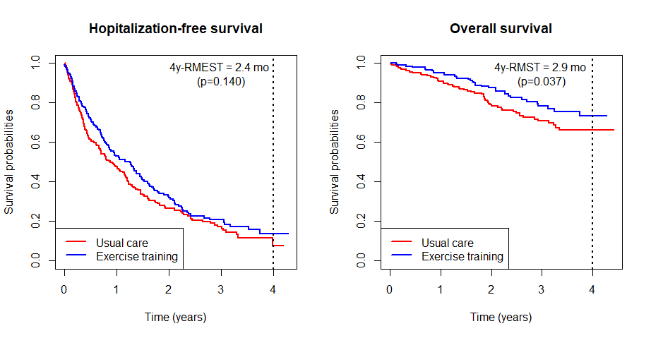
- Traditional composite and overall survival
![]()
R-Code
# fit RMT-IF
obj <- rmtfit(hfaction$patid, hfaction$time, hfaction$status, hfaction$trt,
              type = "recurrent")
summary(obj, Kmax = 4, tau = 3.97) ## combine recurrent events >= 4
# Restricted mean time in favor of group "1" by time tau = 3.97:
#   Estimate    Std.Err Z value Pr(>|z|)
# Event 1   0.0140515  0.0498836  0.2817 0.778184
# Event 2   0.0358028  0.0499618  0.7166 0.473619
# Event 3   0.1385287  0.0409533  3.3826 0.000718 ***
# Event 4+ -0.0064731  0.0600813 -0.1077 0.914203
# Survival  0.2384169  0.1143484  2.0850 0.037069 *
# Overall   0.4203268  0.1777363  2.3649 0.018035 *
Graphics
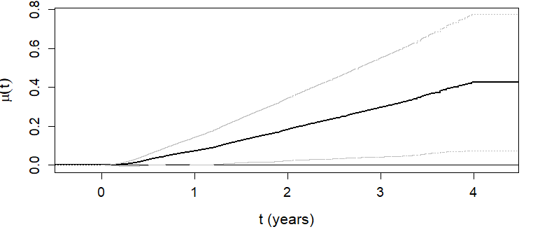
\(\hat\mu(t)\) as a function of \(t\)
- Overall RMT-IF becomes significant after 1 year (see lower CL)
![]()
Inference Results
- 4-year RMT-IF of exercise training
- Training on average gains 5.1 months (\(P\)=0.018) in favorable state
Estimate SE P-value Hopitalization 2.18 1.22 0.073 1 0.17 0.60 0.778 2 0.43 0.60 0.474 3 1.66 0.49 <0.001 4+ -0.08 0.72 0.914 Death 2.86 1.37 0.037 Overall 5.04 2.13 0.018 - 2.9 months net survival \(+\) 2.2 months net time with fewer hospitalizations (little effect on 1st)
Favorability Plot
- 4-year average win-loss times

Summary and Discussion
Summary
- RMT-IF
- A model-free estimand to measure treatment effect on hierarchical composite endpoints
- Net average win time \(=\) Average win \(-\) loss time
- \(\sum_k\) (Net average win time on \(k\)th component)
- R-package:
rmtobj <- rmtfit(id, time, status, trt, type = c("multistate", "recurrent"))summary(obj, tau)plot(obj)
Discussion
- Standard win-loss measures
- Longer survivor wins categorically (on patient-level)
![]()
- Longer survivor wins categorically (on patient-level)
- RMT-IF
Quantitative win-loss times (on patient-time-level)
Loss on nonfatal event can (more than) offset win on survival
- Disregard win/loss time on nonfatal event in presence of death?
Future Topics
- Covariate adjustment
- Conditional estimand \(\to\) regression modeling
- Marginal estimand \(\to\) Augmentation under working regression model (locally efficient estimation)
- Intercurrent event
- Treatment non-response/toxicity/discontinuation (ICH, 2020)
- “occurring after treatment initiation that affect either the interpretation or the existence of the measurements associated with the clinical question of interest”
- How to measure win/loss time afterward?
- Treatment non-response/toxicity/discontinuation (ICH, 2020)
Acknowledgments
Funding
- R01HL149875 (11/2019 – 7/2028)
- DMS2015526 (7/2020 – 6/2024)
![]()
Collaborators
- KyungMann Kim, Tuo Wang, etc.
References
Cook, R. J., & Lawless, J. F. (2018). Multistate models for the analysis of life history data. Chapman; Hall/CRC. https://doi.org/10.1201/9781315119731
Dong, G., Huang, B., Wang, D., Verbeeck, J., Wang, J., & Hoaglin, D. C. (2021). Adjusting win statistics for dependent censoring. Pharmaceutical Statistics, 20(3), 440–450. https://doi.org/10.1002/pst.2086
Dong, G., Mao, L., Huang, B., Gamalo-Siebers, M., Wang, J., Yu, G., & Hoaglin, D. C. (2020b). The inverse-probability-of-censoring weighting (IPCW) adjusted win ratio statistic: an unbiased estimator in the presence of independent censoring. Journal of Biopharmaceutical Statistics, 30(5), 882–899. https://doi.org/10.1080/10543406.2020.1757692
ICH. (2020). ICH E9 (R1) addendum on estimands and sensitivity analysis in clinical trials to the guideline on statistical principles for clinical trials, step 5. London: European Medicines Evaluation Agency.
Mao, L. (2023a). On restricted mean time in favor of treatment. Biometrics, 79(1), 61–72. https://doi.org/10.1111/biom.13570
Mao, L. (2023b). Power and Sample Size Calculations for the Restricted Mean Time Analysis of Prioritized Composite Endpoints. Statistics in Biopharmaceutical Research, 15(3), 540–548. https://doi.org/10.1080/19466315.2022.2110936
Mao, L. (2023c). Study Design for Restricted Mean Time Analysis of Recurrent Events and Death. Biometrics, 79(4), 3701–3714. https://doi.org/10.1111/biom.13923
Mao, L. (2024). Defining estimand for the win ratio: Separate the true effect from censoring. Clinical Trials, 10.1177/17407745241259356.
Mao, L., & Wang, T. (2024). Dissecting the restricted mean time in favor of treatment. Journal of Biopharmaceutical Statistics, 34(1), 111–126. https://doi.org/10.1080/10543406.2023.2210658
Pocock, S. J., Ariti, C. A., Collier, T. J., & Wang, D. (2012). The win ratio: a new approach to the analysis of composite endpoints in clinical trials based on clinical priorities. European Heart Journal, 33(2), 176–182. https://doi.org/10.1093/eurheartj/ehr352


