Applied Survival Analysis
Chapter 5 - Other Non-/Semi-Parametric Methods
Department of Biostatistics & Medical Informatics
University of Wisconsin-Madison
Outline
Restricted Mean Survival Time (RMST)
Additive Hazards (AH) Model
Proportional Odds (PO) Model
Accelerated Failure Time (AFT) Model
\[\newcommand{\d}{{\rm d}}\] \[\newcommand{\T}{{\rm T}}\] \[\newcommand{\dd}{{\rm d}}\] \[\newcommand{\pr}{{\rm pr}}\] \[\newcommand{\var}{{\rm var}}\] \[\newcommand{\se}{{\rm se}}\] \[\newcommand{\indep}{\perp \!\!\! \perp}\] \[\newcommand{\Pn}{n^{-1}\sum_{i=1}^n}\]
Restricted Mean Survival Time (RMST)
Motivation
- Limitations of hazard ratio
- Proportionality
- Depends on time frame in case of non-proportionality
- Alternative metric
- \(\tau\)-year survival rate \(S(\tau)\) for a fixed \(\tau\)
- \(5\)-year survival rates for cancer patients
- \(S_1(\tau) - S_0(\tau)\): increase in survival rate by treatment vs control
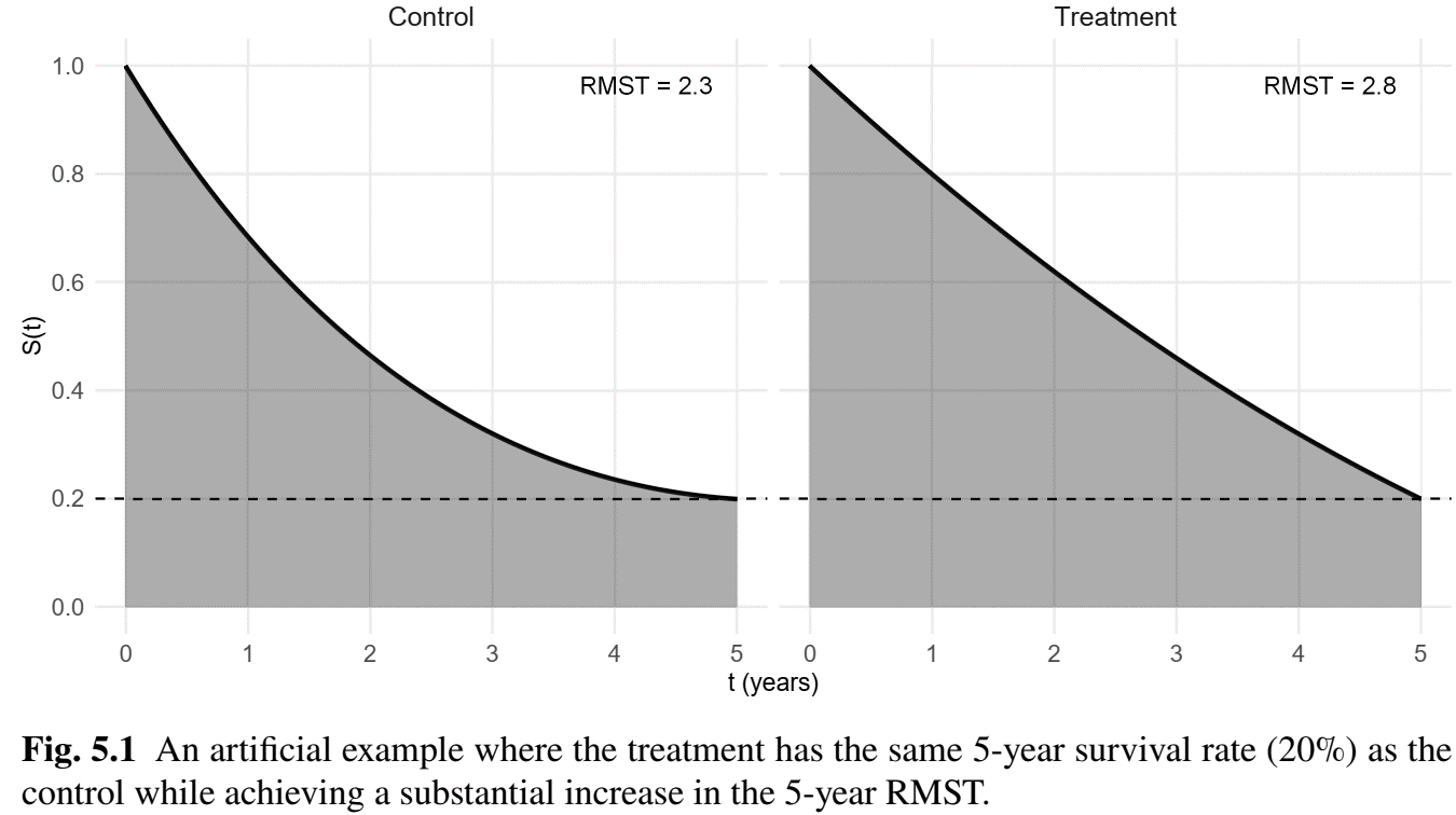
- Limitation: cross-sectional survival status at \(\tau\)
- Distribution of \(T\) in \([0, \tau]\) ignored
- Delay of death within \([0, \tau]\) not captured
- \(\tau\)-year survival rate \(S(\tau)\) for a fixed \(\tau\)
Definition and Interpretation
- Restricted mean survival time (RMST) \[\mu(\tau)=E(T\wedge\tau)\]
- a.k.a. Restricted mean life
- Averaged time lived in the first \(\tau=5\) years
- Restricted mean time lost (RMTL): \(L(\tau) = \tau - \mu(\tau)\)
- Alternate expression (area under survival curve, AUC) \[\begin{equation}\label{eq:non_haz:auc}
\mu(\tau)=\int_0^\tau S(t)\dd t.
\end{equation}\]
- Estimator \(\hat\mu(\tau)=\int_0^\tau \hat S(t)\dd t\), where \(\hat S(t)\) is KM estimator
Survival Rate vs RMST
- \(S(\tau)\) vs \(\mu(\tau)\)
- \(S(\tau)\): survival status at \(\tau\)
- \(\mu(\tau)\): summary of survival experience in \([0, \tau]\) (more information)
Two-Sample Inference
- Effect size (\(a=1\): treatment; 0: control)
- Additive: \(\mu_1(\tau)-\mu_0(\tau)\)
- Average survival (event-free) time gained in \([0, \tau]\)
- Multiplicative: \(\mu_1(\tau)/\mu_0(\tau)\) or \(L_1(\tau)/L_0(\tau)\)
- Fold change in average survival time (lost) in \([0, \tau]\)
- Additive: \(\mu_1(\tau)-\mu_0(\tau)\)
- Estimation and inference
- Plug in KM estimators \(\hat S_a(t)\) \((a= 1, 0)\)
- Obtain \(\hat\var\{\hat\mu_a(\tau)\}\) by \[
\hat\mu_a(\tau) = \mbox{time-weighted sum of the }\hat S_a(t_j)
\mbox{ up to }\tau
\]
- Greenwood’s formula for \(\hat\var\{\hat S_a(t_j)\}\)
Regression Models
- Modeling target: conditional RMST \[ \mu(\tau\mid Z)=E(T\wedge \tau\mid Z) \]
- Model specification \[
g\{\mu(\tau\mid Z)\}=\beta^\T Z
\]
- \(g(x) = x\): Additive model on RMST
- Unit increases in \(Z\) increase \(\tau\)-RMST by \(\beta\)
- \(g(x) = \log(x) \mbox{ or } \log(\tau -x)\): Multiplicative model on RMST/RMTL
- Unit increases in \(Z\) change \(\tau\)-RMST/RMTL by \(\exp(\beta)\) times
- \(Z = 1, 0\) \(\Rightarrow\) Two-sample additive/multiplicative effect sizes
- \(g(x) = x\): Additive model on RMST
Fitting Regression Models
- Observed data
\[ (X_i, \delta_i, Z_i)\,\,\, i=1,\ldots, n \]
Inverse probability censoring weighting (IPCW) \[\begin{equation}\label{eq:nonhaz_rmst_ipcw} n^{-1}\sum_{i=1}^n \frac{\delta_i}{G(X_i\mid Z_i)}Z_i \{X_i\wedge\tau - g^{-1}(\hat\beta^\T Z_i)\} = 0, \end{equation}\]
- \(G(t\mid Z) = \pr(C>t\mid Z)\): replace by model-based version
- Works because \(E\left[\frac{\delta}{G(X\mid Z)}Z\{X\wedge\tau - g^{-1}(\beta^\T Z)\}\right]=0\) under \(C\indep T\mid Z\) (Exercise)
Software: survRM2::rmst2() (I)
- Basic syntax for RMST analysis
- Input
(time, status): \((X, \delta)\)arm: vector of indicators (1-0) for treatment vs controltau: scaler \(\tau\)covariates: optional covariate matrix (or data frame)
Software: survRM2::rmst2() (II)
- Two-sample output (
covariates = NULL)obj$RMST.arm1&obj$RMST.arm0: two lists of group-wise inference results forarm = 1and0obj$unadjusted.result: matrix containing estimates, 95% confidence intervals, and \(p\)-values for \(\mu_1(\tau) - \mu_0(\tau)\), \(\mu_1(\tau)/\mu_0(\tau)\), and \(L_1(\tau)/L_0(\tau)\)
- Regression output (
covariatessupplied)obj$RMST.difference.adjusted: regression results for \(g(x) =x\)obj$RMST.ratio.adjusted: regression results for \(g(x) = \log(x)\)obj$RMTL.ratio.adjusted: regression results for \(g(x) = \log(\tau - x)\)
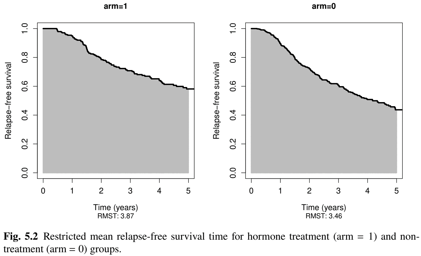
RMST: German Breast Cancer (I)
- Endpoint: 5-year restricted mean relapse-free survival time
- Two-sample: Hormone (
arm=1) vs non-hormone (arm=0)
- Two-sample: Hormone (
# Two sample: hormonal and non-hormonal groups on 5-year RMST
obj <- rmst2(time = df$time / 12, status = df$status,
            arm = df$hormone - 1, tau = 5)
obj
# Restricted Mean Survival Time (RMST) by arm
#              Est.    se lower .95 upper .95
# RMST (arm=1) 3.87 0.104     3.666     4.074
# RMST (arm=0) 3.46 0.084     3.295     3.625
#
# Restricted Mean Time Lost (RMTL) by arm
#              Est.    se lower .95 upper .95
# RMTL (arm=1) 1.13 0.104     0.926     1.334
# RMTL (arm=0) 1.54 0.084     1.375     1.705
RMST: German Breast Cancer (II)
Two-sample
- Hormone increases 5-year RMST by 0.41 years (\(p\)=0.002)
# Between-group contrast
#                       Est. lower .95 upper .95     p
# RMST (arm=1)-(arm=0) 0.410     0.148     0.672 0.002
# RMST (arm=1)/(arm=0) 1.118     1.042     1.201 0.002
# RMTL (arm=1)/(arm=0) 0.734     0.595     0.905 0.004
#
#-----  Graphic -------------------------------------------------
# Graphical display of the group-specific RMST
# as area under the KM curves
plot(obj, xlab="Time (years)", ylab = "Relapse-free survival",
     col.RMST = "gray", col.RMTL = "white", cex.lab = 1.2,
     cex.axis = 1.2, col = "black", xlim = c(0,5))
RMST: German Breast Cancer (III)
- Two-sample
RMST: German Breast Cancer (IV)
- Regression
- Hormone extends 5-year RMST by 1.137 - 1 = 13.7% (\(p<\) 0.001)
# Regression with all the other covariate
obj_reg <- rmst2(time = df$time / 12, status = df$status,
            arm = df$hormone - 1, covariates = df[, 5:11], tau = 5)
#----- Print out multiplicative model on RMST ---------------
obj_reg$RMST.ratio.adjusted
#             coef se(coef)      z     p exp(coef) lower .95 upper .95
# intercept  1.574    0.153 10.257 0.000     4.824     3.571     6.516
# arm        0.129    0.039  3.318 0.001     1.137     1.054     1.227
# age        0.006    0.004  1.537 0.124     1.006     0.998     1.013
# meno      -0.111    0.072 -1.539 0.124     0.895     0.777     1.031
# size      -0.004    0.002 -2.132 0.033     0.996     0.992     1.000
# grade     -0.120    0.035 -3.463 0.001     0.887     0.828     0.949
# nodes     -0.032    0.006 -5.421 0.000     0.969     0.957     0.980
# ...
Additive Hazards (AH) Model
Semiparametric AH Model
- Additive, not multiplicative (Cox), hazards \[\begin{equation}\label{eq:non_haz:add_haz}
\lambda(t\mid Z)=\lambda_0(t)+\beta^\T Z,
\end{equation}\]
- \(\beta_k\): risk difference (attributable risk) with one unit increase in \(Z_{\cdot k}\)
- Unit: per (person-)time
- “Score” equation
- \(\hat\beta\): explicit solution to \(U_n(\hat\beta)=0\) (Lin and Ying, 1994) \[\begin{equation} U_n(\beta) = n^{-1}\sum_{i=1}^n\int_0^\tau\left\{Z_i -\frac{\sum_{j=1}^n I(X_j\geq t)Z_j}{\sum_{j=1}^n I(X_j\geq t)}\right\} \{\dd N_i(t) - I(X_i\geq t)\beta^\T Z_i \dd t\}, \end{equation}\]
AH Model Extensions
- Time-varying covariates \[\begin{equation} \lambda(t\mid Z) =\lambda_0(t)+\beta^\T Z(t) \end{equation}\]
Residuals
- Cox-Snell, score, martingale/deviance
Aalen’s nonparametric AH model \[\begin{equation}\label{eq:non_haz:add_haz1} \lambda(t\mid Z)=\lambda_0(t)+\beta(t)^\T Z(t), \end{equation}\]
- Least-squares type estimates for \(B(t)=\int_0^t\beta(s)\dd s\)
- Can be used to check constancy of \(\beta\)
Software: addhazard::ah()
- Basic syntax for semiparametric AH
- Input
Surv(time, status) ~ covariates: same formula as incoxph()ties = FALSE: specify and de-tietime(add a small noise)
- Output: an object of class
ahobj$coef: \(\hat\beta\),obj$var: \(\hat\var(\hat\beta)\)summary(obj): outputs regression table
Software: timereg::aalen()
- Basic syntax for Aalen’s nonparametric AH
- Input
Surv(time, status) ~ covariates: same formula ascoxph()
- Output: an object of class
aalenobj$cum: matrix containing \(t\) and \(\hat B(t)\)obj$var: matrix containing \(t\) and pointwise \(\hat\var\{\hat B(t)\}\)summary(obj): outputs test results for \(H_0: \beta(t)\equiv 0\)
AH: German Breast Cancer (I)
- Semiparametric AH model
- Hormone reduces relapse/death rate by 0.050 per person-year
# Add a small random number to time to get rid of ties
df$time.dties <- df$time/12 + runif(nrow(df),0, 1e-12)
# fit an additive hazard model
obj <- ah(Surv(time.dties, status) ~ hormone + meno + age + size +
            grade + nodes + prog + estrg, data = df, ties = FALSE)
# print out summary
summary(obj)
#               coef         se   lower.95   upper.95      z  p.value
# hormone -0.0497713  0.0170343 -0.0831585 -0.0163842 -2.922  0.00348 **
# meno     0.0373581  0.0242005 -0.0100749  0.0847911  1.544  0.12266
# age     -0.0011667  0.0013891 -0.0038895  0.0015560 -0.840  0.40096
# size     0.0010200  0.0007299 -0.0004107  0.0024506  1.397  0.16231
# ...
AH: German Breast Cancer (II)
- Semi- vs. Non-parametric

Proportional Odds (PO) Model
Semiparametric PO Model
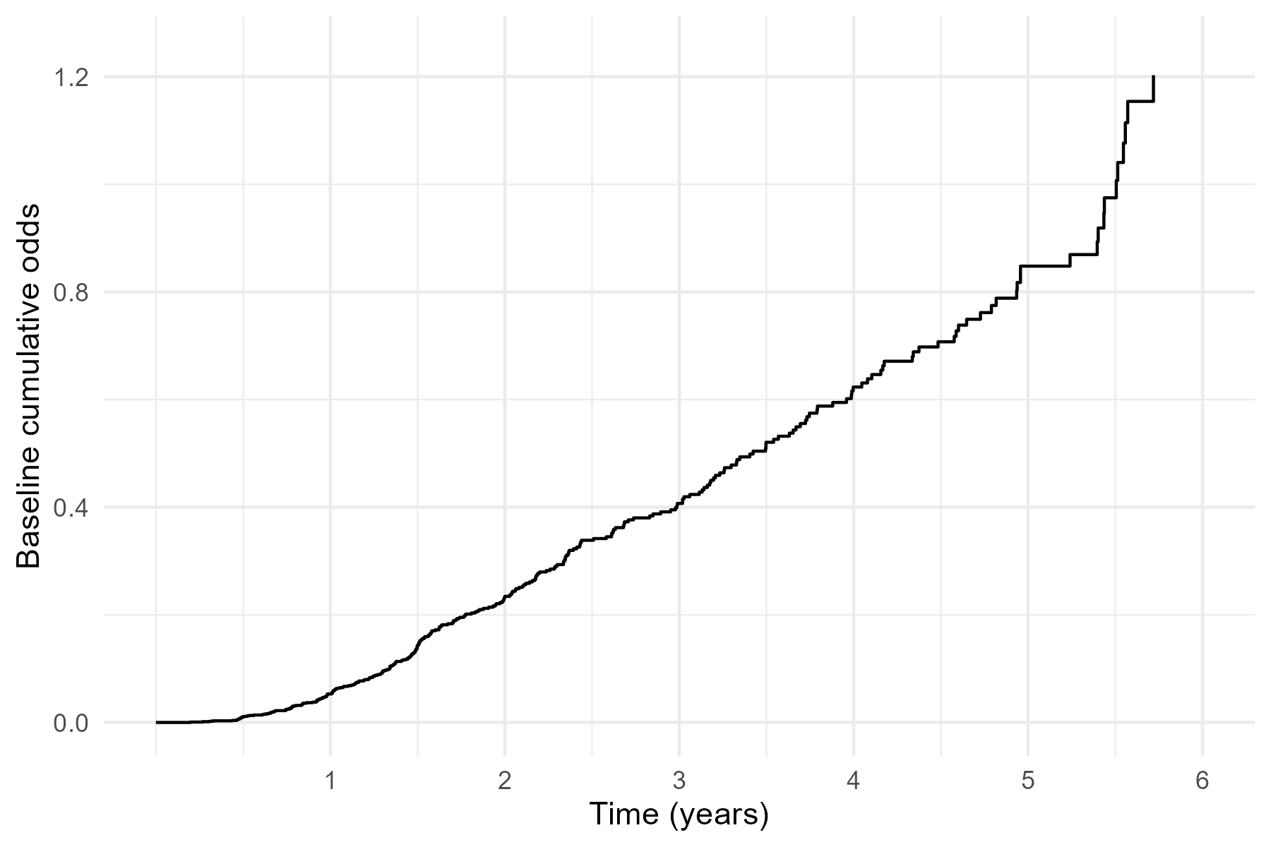
- Model specification \[\begin{equation}\label{eq:non_haz:po}
\log\left\{\frac{1-S(t\mid Z)}{S(t\mid Z)}\right\}=h_0(t)+\beta^\T Z,
\end{equation}\]
- \(h_0(t)\): nonparametric (non-decreasing) baseline cumulative log-odds
- Fix \(t\) \(\to\) logistic regression for \(I(T\leq t)\)
- Time-varying intercept, constant odds ratio
- Proportional odds \[\begin{equation}\label{eq:non_haz:poprop}
\frac{\{1-S(t\mid z_1)\}/S(t\mid z_1)}{\{1-S(t\mid z_2)\}/S(t\mid z_2)}=\exp\{\beta^\T(z_1-z_2)\}.
\end{equation}\]
- \(\exp(\beta_k)\): odds ratio for an early event (regardless of cut-off) with one unit increase in \(Z_{\cdot k}\)
Estimation and Extension
- Estimation and inference
- Nonparametric MLE: Joint maximization w.r.t. \(\beta\) and the \(\Delta h(t_j)= h(t_j) - h(t_j-)\) \((j=1,\ldots, m)\)
- Semiparametric transformation models \[\begin{equation}\label{eq:non_haz:linear_trans}
g\{F(t\mid Z)\}=h_0(t)+\beta^\T Z,
\end{equation}\]
- \(F(t\mid Z)=1- S(t\mid Z)\)
- \(\log\{x/(1-x)\}\): Proportional odds
- \(\log(-\log(1 - x))\): Proportional hazards (Cox)
Software: timereg::prop.odds()
- Basic syntax for semiparametric PO model
- Input
Event(time, status) ~ covariates: similar toSurv(time, status) ~ covariatesincoxph()
- Output: an object of class
cox.aalenobj$gamma: \(\hat\beta\);obj$var.gamma: \(\hat\var(\hat\beta)\)obj$cum: matrix containing \(t\) and \(\exp\{\hat h_0(t)\}\)summary(obj): summarizes regression results
PO: German Breast Cancer (I)
- Semiparametric PO model
- Hormone reduces odds of early relapse/death by \(1-\exp(-0.522)=40.7\%\) (\(p\)-value 0.002)
# Fit a PO model
obj <- prop.odds(Event(time, status) ~ hormone + meno + age + size +
                   grade + nodes + prog + estrg, data = df)
# print out summary
summary(obj)
#              Coef.  SE       z      P-val   lower2.5% upper97.5%
# hormone2 -0.52200 0.17000  -3.0800 2.08e-03 -0.855000   -0.18900
# meno2     0.49000 0.24300   1.9100 5.66e-02  0.013700    0.96600
# age      -0.02240 0.01280  -1.7500 8.09e-02 -0.047500    0.00269
# size      0.01150 0.00611   1.7800 7.57e-02 -0.000475    0.02350
# ...
PO: German Breast Cancer (II)
Accelerated Failure Time (AFT) Model
Model Specification
- Log-linear model \[\begin{equation}\label{eq:non_haz:aft}
\log T=\beta^\T Z + \epsilon, \hspace{10mm} \epsilon\indep Z,
\end{equation}\]
- \(\epsilon\): random error with unknow distribution
- \(T=\exp(\beta^\T Z)\exp(\epsilon)\): multiplicative covariate effects on \(T\)
- \(Z\) changes survival time by \(\exp(\beta^\T Z)\) fold
- Accelerated failure time (AFT): with \(S_\epsilon(t)=\pr\{\exp(\epsilon) > t\}\) \[\begin{align*}
S(t\mid Z) &=\pr\left\{\exp(\beta^\T Z)\exp(\epsilon) > t\mid Z\right\}\\
& = S_\epsilon\left\{\exp(-\beta^\T Z)t\right\}
\end{align*}\]
- Accelerates time course by a factor of \(\exp(\beta^\T Z)\)
Parametric vs Semiparametric
- Parametric AFT
- \(\exp(\epsilon)\sim\) Weibull, log-normal, log-logistic, etc
- Simplifies estimation \(\to\) MLE
- Weibull AFT model \(\Leftrightarrow\) Weibull PH model (only distribution with this equivalency)
- Semiparametric AFT
- \(\exp(\epsilon)\sim\) nonparametric distribution
- Buckley-James estimator \[ \mbox{Least squares} \stackrel{\rm iterate}{\longleftrightarrow} \mbox{Imputing censored values} \]
Software: aftgee::aftgee()
- Basic syntax for semiparametric AFT model
- Input
Surv(time,status) ~ covariates: same formula as incoxph()
- Output: an object of class
aftgeeobj$coef.res: \(\hat\beta\)obj$var.res: \(\hat\var(\hat\beta)\)summary(obj): summarizes regression results
AFT: German Breast Cancer
- Semiparametric AFT model
- Hormone increases relapse-free survival time by \(\exp(0.320) = 1.38\) fold (\(p\)-value 0.001)
# Fit an AFT model
set.seed(123)  # SE is based on resampling
obj <- aftgee(Surv(time, status) ~ hormone + meno + age + size + grade +
                nodes + prog + estrg, data = df,
                B = 500) # Number of resamples
# print out summary
summary(obj)
#             Estimate StdErr z.value p.value
# (Intercept)    4.262  0.410   10.40  <2e-16 ***
# hormone2       0.320  0.092    3.47   0.001 ***
# meno2         -0.270  0.148   -1.82   0.068 .
# age            0.013  0.007    1.69   0.092 .
# size          -0.006  0.003   -1.89   0.059 .
# ...
Conclusion
Notes
- Pseudo-value approach to RMST regression \[
\hat{\mu}_i(\tau) = n \hat{\mu}(\tau) - (n - 1) \hat{\mu}^{(-i)}(\tau)
\]
- \(\hat{\mu}^{(-i)}(\tau)\): RMST without \(i\)-th observation
- Regress \(\hat{\mu}_i(\tau)\) on \(Z_i\)
pseudopackage
- Cox–Aalen model \[
\lambda(t \mid Z) \;=\; \lambda_0(t) \exp\left(\gamma^\T Z_{(1)}\right) + \beta(t)^\T Z_{(2)}
\]
- Multiplicative hazards for \(Z_{(1)}\), additive hazards for \(Z_{(2)}\)
timereg::cox.aalen()
Summary (I)
- \(\tau\)-RMST
- Difference/ratio in survival time by time \(\tau\)
- Two-sample and regression
survRM2::rmst2()
- Additive hazards
- Difference in risk (attributable risk)
addhazard::ah()(semiparametric: constant difference)timereg::aalen()(nonparametric: time-varying difference)
Summary (II)
- Proportional odds
- Odds ratio for an early event
timereg::prop.odds()
- Accelerated failure time
- Ratio in survival time
aftgee::aftgee()(semiparametric: unspecified error distribution)survival::survreg()(parametric error distribution)