
| Metric | Range | Focus | Time.Dimension | Affected.by.Censoring |
|---|---|---|---|---|
| Harrell’s C | [0, 1] | Discrimination | Overall | Yes |
| Uno’s C_tau | [0, 1] | Discrimination | Overall | No |
| Time-dependent AUC(t) | [0, 1] | Discrimination | Dynamic | No |
| Integrated AUC | [0, ∞) | Discrimination | Overall | No |
| Brier score BS(t) | [0, ∞) | Discrimination/Calibration | Dynamic | No |
| Integrated Brier score | [0, ∞) | Discrimination/Calibration | Overall | No |
Applied Survival Analysis
Chapter 15 - Machine Learning in Survival Analysis
Lu Mao
Department of Biostatistics & Medical Informatics
University of Wisconsin-Madison
Outline
Regularized Cox regression models
Survival trees and random forests
Survival surport vector machines
R’s Tidymodels system
\[\newcommand{\d}{{\rm d}}\] \[\newcommand{\T}{{\rm T}}\] \[\newcommand{\dd}{{\rm d}}\] \[\newcommand{\cc}{{\rm c}}\] \[\newcommand{\pr}{{\rm pr}}\] \[\newcommand{\var}{{\rm var}}\] \[\newcommand{\se}{{\rm se}}\] \[\newcommand{\indep}{\perp \!\!\! \perp}\] \[\newcommand{\Pn}{n^{-1}\sum_{i=1}^n}\] \[ \newcommand\mymathop[1]{\mathop{\operatorname{#1}}} \] \[ \newcommand{\Ut}{{n \choose 2}^{-1}\sum_{i<j}\sum} \]
Regularized Cox Regression
Rationale
- With many covariates
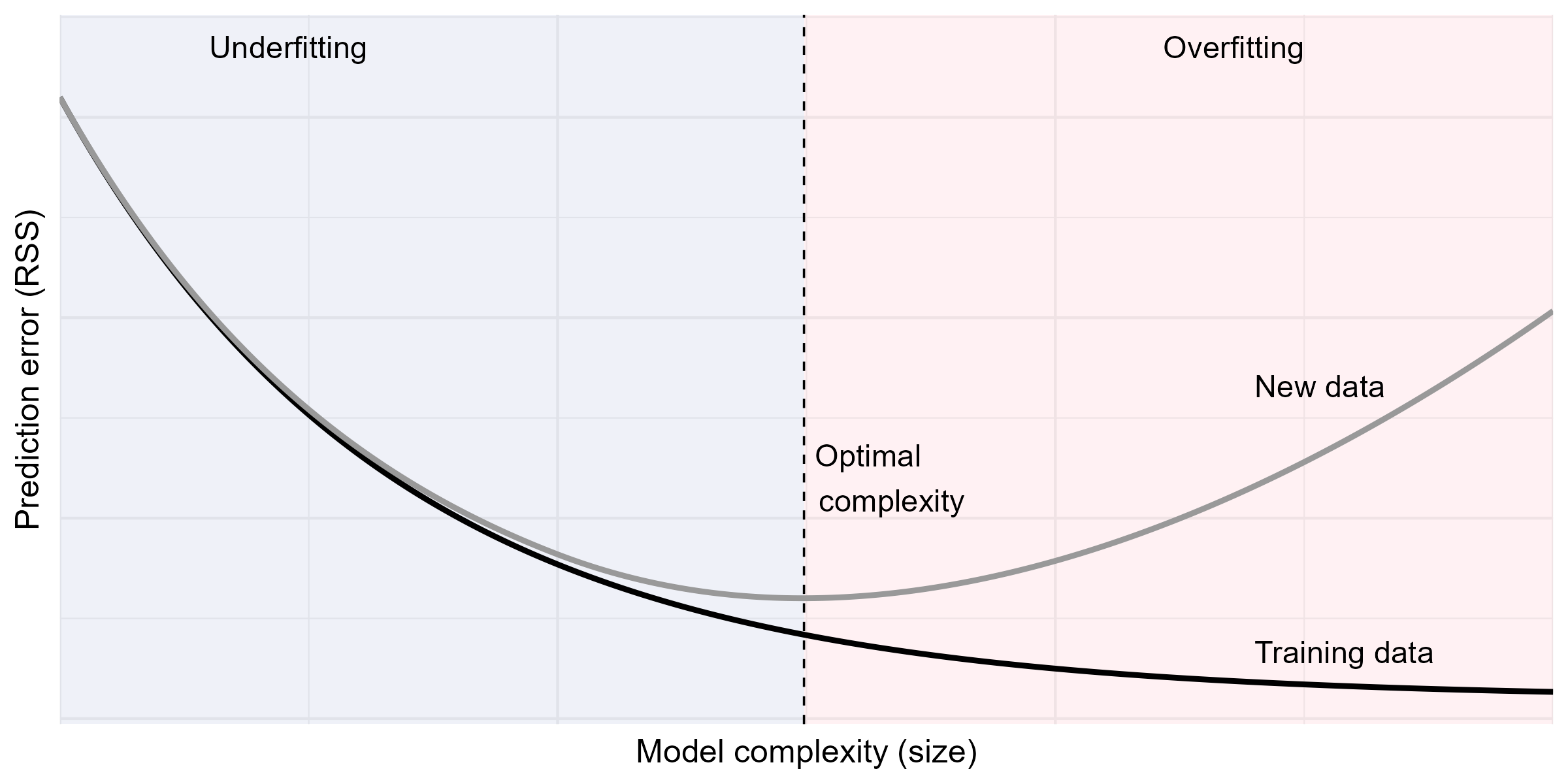
- Prediction accuracy: under- vs over-fitting
![]()
- Too many predictors \(\to\) overfitting
- Interpretation: easier with fewer predictors
- Prediction accuracy: under- vs over-fitting
Linear Model Basics
- Set-up \[
Y=\alpha+\beta^\T Z+\epsilon
\]
- \(Z\): a \(p\)-vector of covariates (predictors)
- \(E(\epsilon\mid Z)=0\)
- Assume WLOG \(\sum_{i=1}^n Y_i=0\) and \(\sum_{i=1}^n Z_i=0\)
- Ordinary least-squares (OLS) estimator \[\begin{align*}
\hat\beta_{\rm OLS}=\arg\min_\beta R_n(\beta)=\left(\sum_{i=1}^n Z_i^{\otimes 2}\right)^{-1}\sum_{i=1}^nZ_iY_i
\end{align*}\]
- \(R_n(\beta)=\sum_{i=1}^n(Y_i-\beta^\T Z_i)^2\): residual sum of squares (RSS)
Subset Selection
- Big \(p\) problem
- Large variance (overfit) \(\to\) poor prediction
- \(p>n\): no fit
- Best-subset selection
- For each \(l\in\{0, 1,\ldots, p\}\), choose best model with \(l\) covariates with least RSS
- \((p+1)\) best models with decreasing RSS (as \(l=0,1,\ldots, p\))
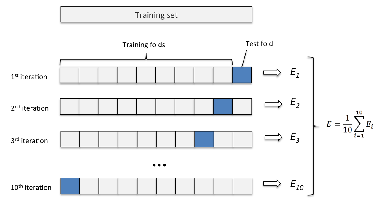
- Choose \(l\) by cross-validation
- Partition sample into \(k\) pieces
- Set one piece aside to evaluate RSS of model fit on remaining data
- Cycle through all \(k\) pieces and average validation errors
Cross-Validation
- Computing validation error
Training vs Prediction Errors
- Typical relationship between training and validation errors
Subset Selection: Limitations
- Best subset
- Fit all \(2^p\) submodels
- Forward/backward stepwise selections
- Start with null/full model, add/drop most/least significant predictor
- Where to stop \(\to\) cross-validation
- Disadvantages
- Computationally costly
- A discrete process: covariates are either retained or dropped; may be sub-optimal for prediction
Penalized Regression (I)
- Constrained least-squares
- Restricting \(L_q\)-norm of \(\beta\) reduces effective d.f. \[\begin{equation}\label{eq:vs:constrained} \tilde\beta(c)=\arg\min_\beta R_n(\beta), \mbox{ subject to }\sum_{j=1}^p|\beta_j|^q\leq c, \end{equation}\]
- Equivalent form by Lagrange multiplier
- \(L_q\)-penalized regression \[\begin{equation}\label{eq:vs:penal}
\hat\beta(\lambda)=\arg\min_\beta \left\{R_n(\beta)+\lambda\sum_{j=1}^p|\beta_j|^q\right\}
\end{equation}\]
- \(\lambda\geq 0\): tuning parameter controlling degree of regulation, determined by cross-validation
- \(\hat\beta(0)=\hat\beta_{\rm OLS}\); \(\hat\beta(\infty)=0\)
- \(L_q\)-penalized regression \[\begin{equation}\label{eq:vs:penal}
\hat\beta(\lambda)=\arg\min_\beta \left\{R_n(\beta)+\lambda\sum_{j=1}^p|\beta_j|^q\right\}
\end{equation}\]
Penalized Regression (II)
- Examples
- Ridge regression \((q=2)\) \[\begin{equation}\label{eq:vs:ridge} \hat\beta(\lambda)=\left(\sum_{i=1}^n Z_i^{\otimes 2}+\lambda I_p\right)^{-1}\sum_{i=1}^nZ_iY_i \end{equation}\]
- Lasso (\(q=1\); Least absolute shrinkage and selection operator)
- Sets some \(\hat\beta_j\equiv 0\); sparse solution
- Elastic net \[\begin{equation}\label{eq:vs:en}
\hat\beta(\lambda)=\arg\min_\beta \left[R_n(\beta)+\lambda\sum_{j=1}^p\left\{\alpha|\beta_j|+2^{-1}(1-\alpha)\beta_j^2\right\}\right]
\end{equation}\]
- Combines the strengths of ridge regression and lasso
- Handles correlated covariates better than lasso
Penalized Regression (III)
- Geometric intuition

Regularized Cox Models
- Unique features with Cox model
- Objective function (RSS not computable due to censoring)
- Computational algorithm
- Definition of error for cross-validation
- Objective function: negative log-partial likelihood \[\begin{equation}\label{eq:vs:cox_lasso}
Q_n(\beta;\lambda)
\;=\;
-\, pl_n(\beta)
\,+\,
\lambda \sum_{j=1}^p
\left\{
\alpha\, |\beta_j|
\,+\,
2^{-1} (1-\alpha)\beta_j^2
\right\}.
\end{equation}\]
- Solution: \(\hat\beta(\lambda)=\arg\min_\beta Q_n(\beta;\lambda)\)
Pathwise Solution
- \(\hat\beta(\lambda)\) as a path of \(\lambda\)
- Iterative \(pl_n(\beta)\approx\) weighted sum of squares
- Coordinate descent (Section 15.1.4 of book chapter)
- \(K\)-fold cross-validation to select \(\lambda_{\rm opt}\)
- Some \(\hat\beta_j(\lambda_{\rm opt})=0\)
- Selected variables \(\{Z_{\cdot j}: \hat\beta_j(\lambda_{\rm opt})\neq 0, j=1,\ldots, p\}\)
Cross-Validation Error
- What is measure of error?
- RSS not applicable due to censoring
- Negative partial-likelihood?
- Unstable with small validation set (risk set too small)
- Partial-likelihood deviance
- On \(j\)th validation set \[
\mbox{CV}_j(\lambda)=pl_{n,-j}\{\hat\beta(\lambda)\}-pl_{n}\{\hat\beta(\lambda)\}
\]
- \(pl_{n,-j}(\beta)\): log-partial likelihood based on training set
- \(\mbox{CV}(\lambda)=k^{-1}\sum_{j=1}^k\mbox{CV}_j(\lambda)\)
- On \(j\)th validation set \[
\mbox{CV}_j(\lambda)=pl_{n,-j}\{\hat\beta(\lambda)\}-pl_{n}\{\hat\beta(\lambda)\}
\]
Testing Model Performance
- Workflow
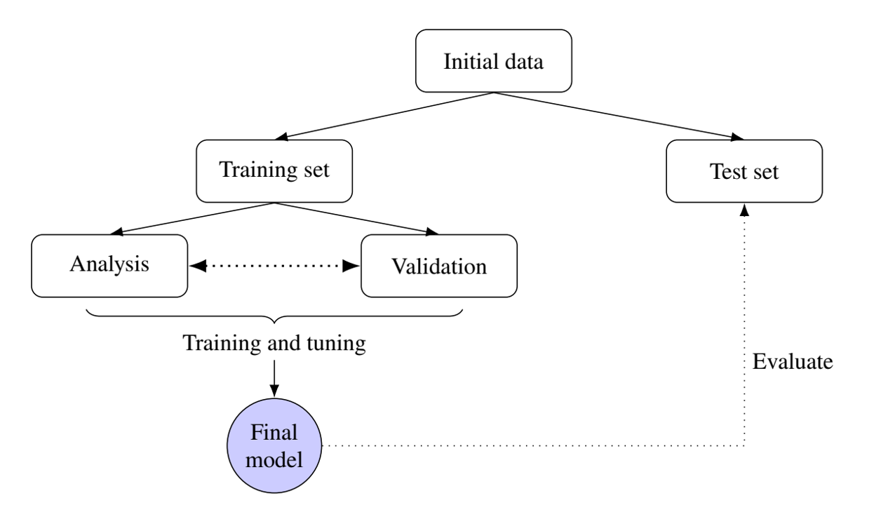
Model Evaluation
- Test data \[
(X_i^*,\, \delta_i^*,\, Z_i^*), \qquad i = 1,\ldots, n^*,
\]
- \(T^*\): true event time
- \(X^* = T^* \wedge C^*\), \(\delta^* = I(T^* \le C^*)\)
- Prediction
- \(\hat g(Z^*)\): predicted risk score (e.g., linear predictor \(\hat\beta^\T Z^*\))
- \(\hat S(t\mid Z^*)\): predicted survival function
Evaluation Metrics - C-Index
- C-index: probability of concordance \[ \mathcal C \;=\; \pr\{ \hat g(Z_i^*) \,>\, \hat g(Z_j^*) \mid T_i^* < T_j^* \} \]
- Harrell’s C-statistic
- Proportion of concordant pairs among comparable pairs \[ \frac{ \sum_{i<j}\sum \delta_i^* I\{ \hat g(Z_i^*) > \hat g(Z_j^*),\, X_i^* < X_j^*\} }{ \sum_{i<j}\sum \delta_i^* I( X_i^* < X_j^*) } \]
- Uno’s C-statistic
- IPCW estimator of probability of concordance by time \(\tau\) \[ \mathcal C_\tau \;=\; \pr\{ \hat g(Z_i^*) > \hat g(Z_j^*) \mid T_i^* < T_j^* \wedge \tau \} \]
Evaluation Metrics - AUC & Brier Score
- AUC: area under the time-dependent ROC curve
- IPCW estimator of probability of concordance at time \(t\) \[ \text{AUC}(t) \;=\; \pr\{ \hat g(Z_i^*) > \hat g(Z_j^*) \mid T_i^* \le t,\; T_j^* > t\} \]
- Brier score
- IPCW estimator mean squared error for predicted vs observed \[ \text{BS}(t) \;=\; E\left[ \left\{ I(T_i^* > t) - \hat S(t \mid Z_i^*) \right\}^2 \right]. \]
Evaluation Metrics - Summary
- Summary of evaluation metrics
Software: glmnet::glmnet() (I)
- Basic syntax for regularized Cox model
- Elastic net \[ \hat\beta(\lambda)=\arg\min_\beta \left[-n^{-1}pl_n(\beta)+\lambda\sum_{j=1}^p\left\{\alpha|\beta_j|+2^{-1}(1-\alpha)\beta_j^2\right\}\right] \]
Z: covariate matrix;alpha: \(\alpha\)
Software: glmnet::glmnet() (II)
- Find optimal \(\lambda\)
- Prediction on test data
beta: \(\hat g(z^*)=\hat\beta^\T z^*\)- Refit Cox model using selected predictors to get \(\hat S(t\mid z^*)\)
GBC: An Example
- German Breast Cancer (GBC) study
- Cohort: 686 breast cancer patients
- Outcome: relapse-free survival
- Predictors: age (\(\leq\) 40 vs >40), menopausal status, hormone treatment, tumor grade, tumor size, lymph nodes, estrogen and progesterone receptor levels
- Training set (\(n=400\)) + test set (\(n^*=286\))
- Cohort: 686 breast cancer patients
Graphics
- Pathwise solution and CV curve
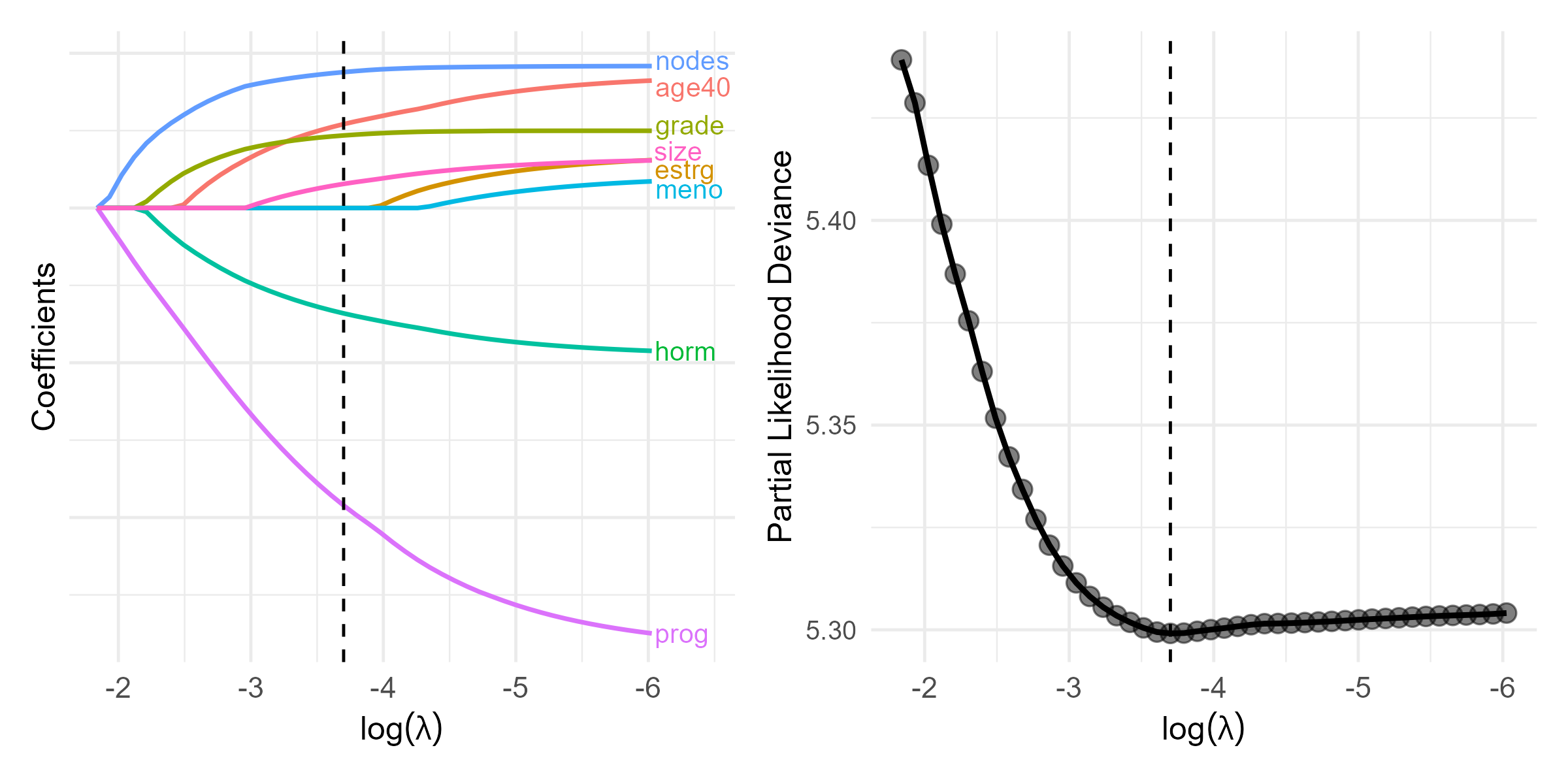
Selected Predictors
CV results
- \(\log(\lambda_{\rm opt}) = -3.7\)
# Identify the optimal lambda
lambda.opt <- obj.cv$lambda.min
lambda.opt
# [1] 0.02472102

# Extract coefficients at lambda.min
beta.opt   <- coef(obj.cv, s = "lambda.min")
# Identify which coefficients are non-zero
beta.selected  <- beta.opt[abs(beta.opt[, 1]) > 0, ]
beta.selected  # show non-zero variables
#>      hormone        age40         size        grade        nodes         prog
#> -0.354175646  0.428284913  0.003006433  0.197080456  0.039587219 -0.002741544
Survival Trees & Random Forests
Decision Trees
- Limitations of regularized Cox model
- Proportionality
- Linearity of covariate effects
- Interactions
- Tree-based classification and regression
- Classification and Regression Trees (CART; Breiman et al., 1984)
- Root node (all sample) \(\stackrel{\rm covariates}{\rightarrow}\) split into (more homogeneous) daughter nodes \(\stackrel{\rm covariates}{\rightarrow}\) split recursively
Basic Procedures
- Growing the tree
- Starting with root node, search splitting criteria \[Z_{\cdot j}\leq z \,\,\,(j=1,\ldots, p; z \in\mathbb R)\] for one that minimizes “impurity” within daughter nodes \[\begin{equation}\label{eq:tree:nodes} A=\{i=1,\ldots, n: Z_{ij}\leq z\} \mbox{ and } B=\{i=1,\ldots, n: Z_{ij}> z\} \end{equation}\]
- Recursive splitting until terminal nodes sufficiently “pure” in outcome
- Tree-based prediction
- A new covariate vector \(\to\) terminal node it belongs \(\to\) predicted outcome
- Majority class
- empirical mean
- Kaplan-Meier estimator
- A new covariate vector \(\to\) terminal node it belongs \(\to\) predicted outcome
An Example
- An illustrative decision tree
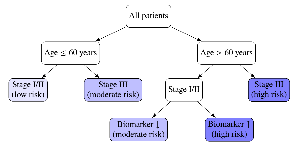
Splitting Criterion
- Objective function
- Choose partition \(A|B\) to minimize \[
R(A\mid\mid B)=\hat P(A)\hat{\mathcal G}(A)+\hat P(B)\hat{\mathcal G}(B)
\]
- \(\hat P(A)\), \(\hat P(B)\): proportions of observations in daughter nodes
- \(\hat{\mathcal G}(A)\), \(\hat{\mathcal G}(B)\): impurity measures within daughter nodes
- Choose partition \(A|B\) to minimize \[
R(A\mid\mid B)=\hat P(A)\hat{\mathcal G}(A)+\hat P(B)\hat{\mathcal G}(B)
\]
- Impurity measure
- Categorical \(Y \in\{1,\ldots, K\}\): Gini index \(\pr(Y_i\neq Y_j)\)
- Continuous: mean squared error
- Survival: mean squared deviance residuals (Cox model with binary node) \[\begin{equation}\label{eq:tree:deviance} R(A\mid\mid B)=n^{-1}\sum_{i \in A}d_{i}^2 +n^{-1}\sum_{i \in B}d_{i}^2 \end{equation}\]
Pruning the Tree
- Penalize complexity
- Cut overgrown branches \(\to\) prevent overfitting \(\to\) generalizability
- Minimize \(R(\mathcal T;\lambda)=R(\mathcal T)+\lambda|\mathcal T|\)
- \(R(\mathcal T)\): mean squared (deviance) residuals for terminal nodes of tree \(\mathcal T\)
- \(|\mathcal T|\): number of terminal nodes
- \(\lambda\geq 0\): cost-complexity parameter determined by cross-validation
- Cut overgrown branches \(\to\) prevent overfitting \(\to\) generalizability
- Final tree
- \(\mathcal T^{\rm opt} = \arg\min_{\mathcal T}R(\mathcal T;\lambda_{\rm opt})\)
- \(\mathcal T^{\rm opt}(z)\): terminal node for new covariate vector \(z\)
- \(\hat S(t\mid z^*)\): KM estimates in node \(\mathcal T^{\rm opt}(z^*)\)
Bagging and Random Forests
- Bagging
- A single tree \(\to\) large variance
- Take \(B\) bootstrapped samples from training data
- \(\mathcal T_b\): survival tree grown on \(b\)th bootstrap sample \((b=1, \ldots, B)\) (without pruning)
- \(\hat S_b(t\mid z)\): predicted survival function
- Final prediction \[ \hat S(t\mid z)=B^{-1}\sum_{b=1}^B \hat S_b(t\mid z) \]
- Random forests
- Same except only a random subset of covariates are considered at each split
- De-correlate the trees grown on different bootstrapped samples)
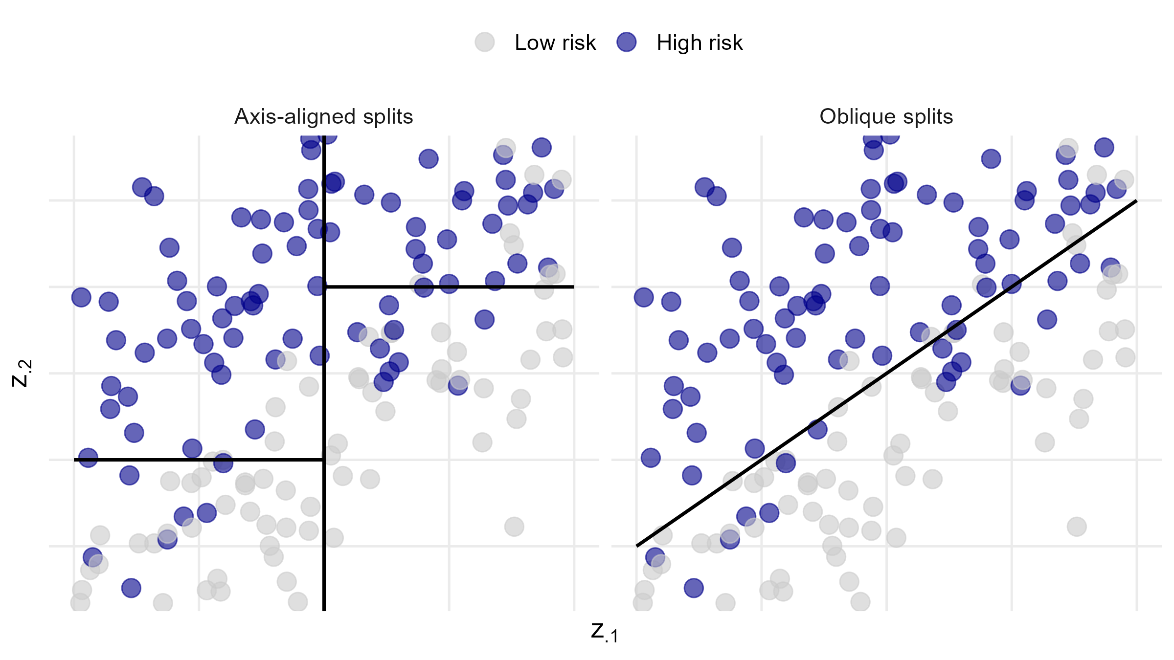
Oblique vs Axis-Aligned Splits
- Split on linear combination of covariates (oblique)
![]()
Out-of-Bag (OOB) Samples
- OOB samples
- \((1-n^{-1})^n\approx 36.8\%\) not included in bootstrap sample for each tree \(\mathcal T_b\)
- Used to compute predictor error
- Monitor performance as forest grows
Software: rpart::rpart()
- Basic syntax for growing survival tree
xval: number of cross-validation foldsminbucket: minimum number of observations in terminal nodescp: complexity parameter (set to 0 for full tree)
# grow the tree, with cross-validation
obj <- rpart(Surv(time, status) ~ covariates,
    control = rpart.control(xval = 10, minbucket = 2, cp = 0))
# cross-validation results
cptable <- obj$cptable
# complexity parameter (lambda)
CP <- cptable[, 1]
# find optimal parameter
# cptable[, 4]: error function
cp.opt <- CP[which.min(cptable[, 4])]
Software: rpart::prune()
- Basic syntax for pruning survival tree
tree:rpartobject for grown tree;cp: optimal \(\lambda\)test: test data frame
# prune the tree, with optimal lambda
fit <- prune(tree = obj, cp = cp.opt)
# plot the pruned tree structure
rpart.plot(fit)
# fit$where: vector of terminal node for training data
# compute KM estimates by terminal node
km <- survfit(Surv(time, status) ~ fit$where)

## prediction on test data ---------------------------
# terminal node for test data
treeClust::rpart.predict.leaves(fit, test)
Software: aorsf:orsf() (I)
- Oblique random survival forests
mtry: number of covariates randomly selected at each split
library(aorsf)
# Fit a basic oblique random survival forest on training data
set.seed(12345) # for reproducibility
fit <- orsf(
  Surv(<time>, <status>) ~ covariates,
  # Optional arguments:
      # Forest size
        n_tree = 500,
      # Number of covariates randomly selected at each split
        mtry = ceiling(sqrt(p)),
         ...
)
Software: aorsf:orsf() (II)
- Variable importance
- Based on degradation of OOB prediction accuracy after permuting \(Z_{\cdot j}\)
- Prediction
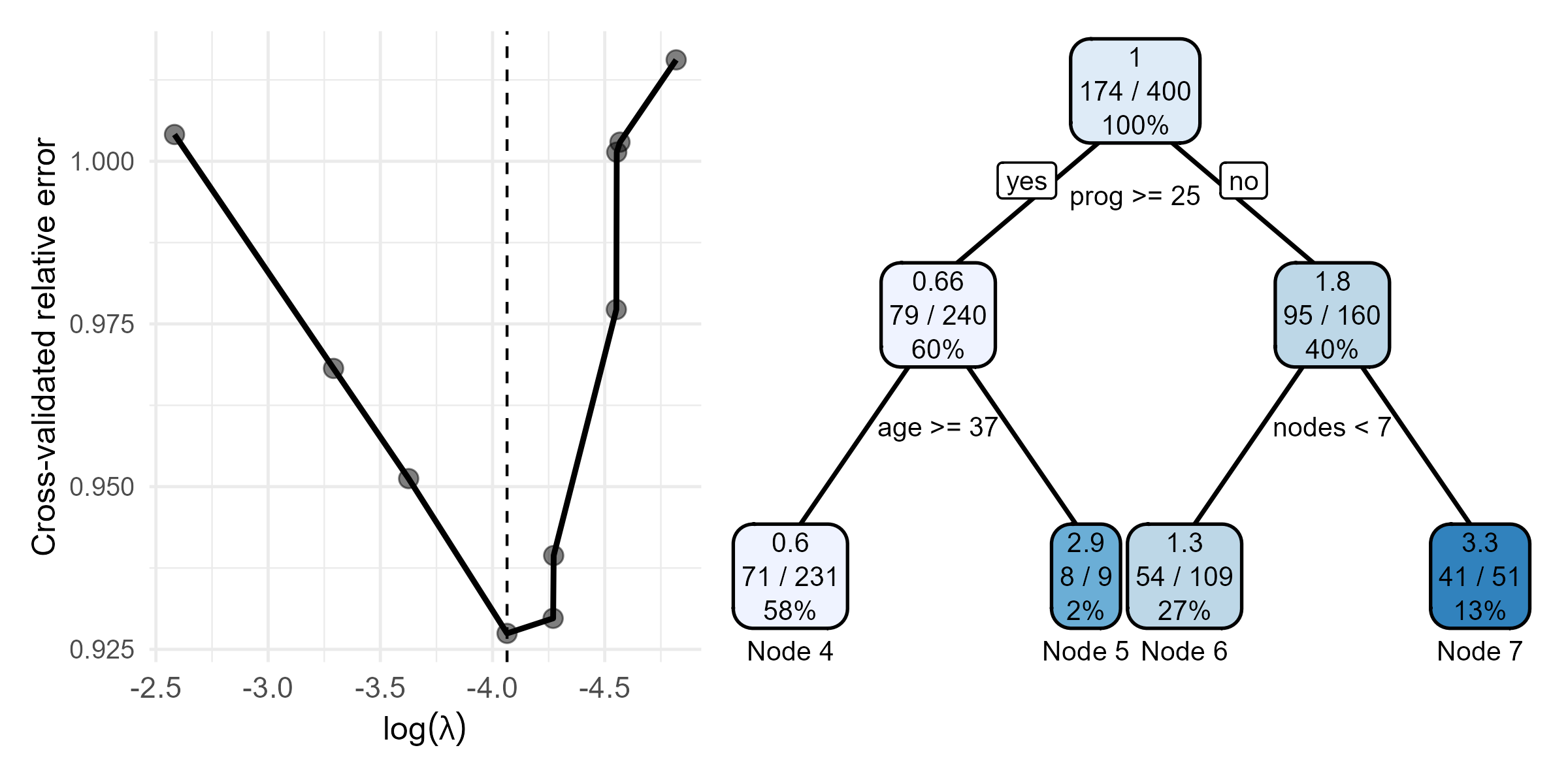
GBC: Fitting Survival Trees
- Same training data
- \(\lambda_{\rm opt}=0.017\); 3 splits (4 terminal nodes)
# Conduct 10-fold cross-validation (xval = 10)
obj <- rpart(Surv(time, status) ~ hormone + meno + size + grade + nodes +
              prog + estrg + age,
             control = rpart.control(xval = 10, minbucket = 2, cp = 0),
             data = train)
printcp(obj) # xerror: objective
#            CP  nsplit rel.error  xerror   xstd
# 1  0.07556835      0   1.00000 1.00411 0.046231
# 2  0.03720019      1   0.92443 0.96817 0.047281
# 3  0.02661914      2   0.88723 0.95124 0.046567
# 4  0.01716925      3   0.86061 0.92745 0.046606 # minimizer
# 5  0.01398306      4   0.84344 0.92976 0.047514
# 6  0.01394869      5   0.82946 0.93941 0.048404
# 7  0.01055028      9   0.77120 0.97722 0.052133
GBC: Survival Tree CV Result
- CV results and final tree
- \(\log(\lambda_{\rm opt}) = -4.1\)
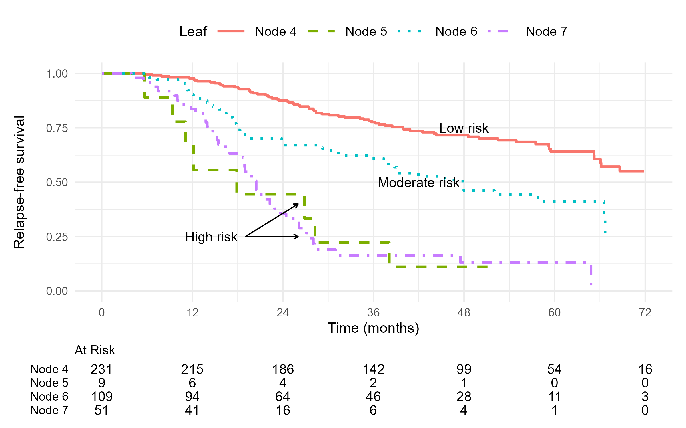
GBC: KM Curves by Terminal Node
- Final tree
GBC: Random Survival Forests
- Fitting RSF
orsf_fit <- orsf(
Surv(time, status) ~ hormone + age + meno + size + grade + nodes + prog + estrg,
data = train,
n_tree = 200,
...
)
print(orsf_fit)
#> ---------- Oblique random survival forest
#> Linear combinations: Accelerated Cox regression
#> N observations: 400
#> N events: 174
#> N trees: 200
#> N predictors total: 8
#> N predictors per node: 3
#> ...
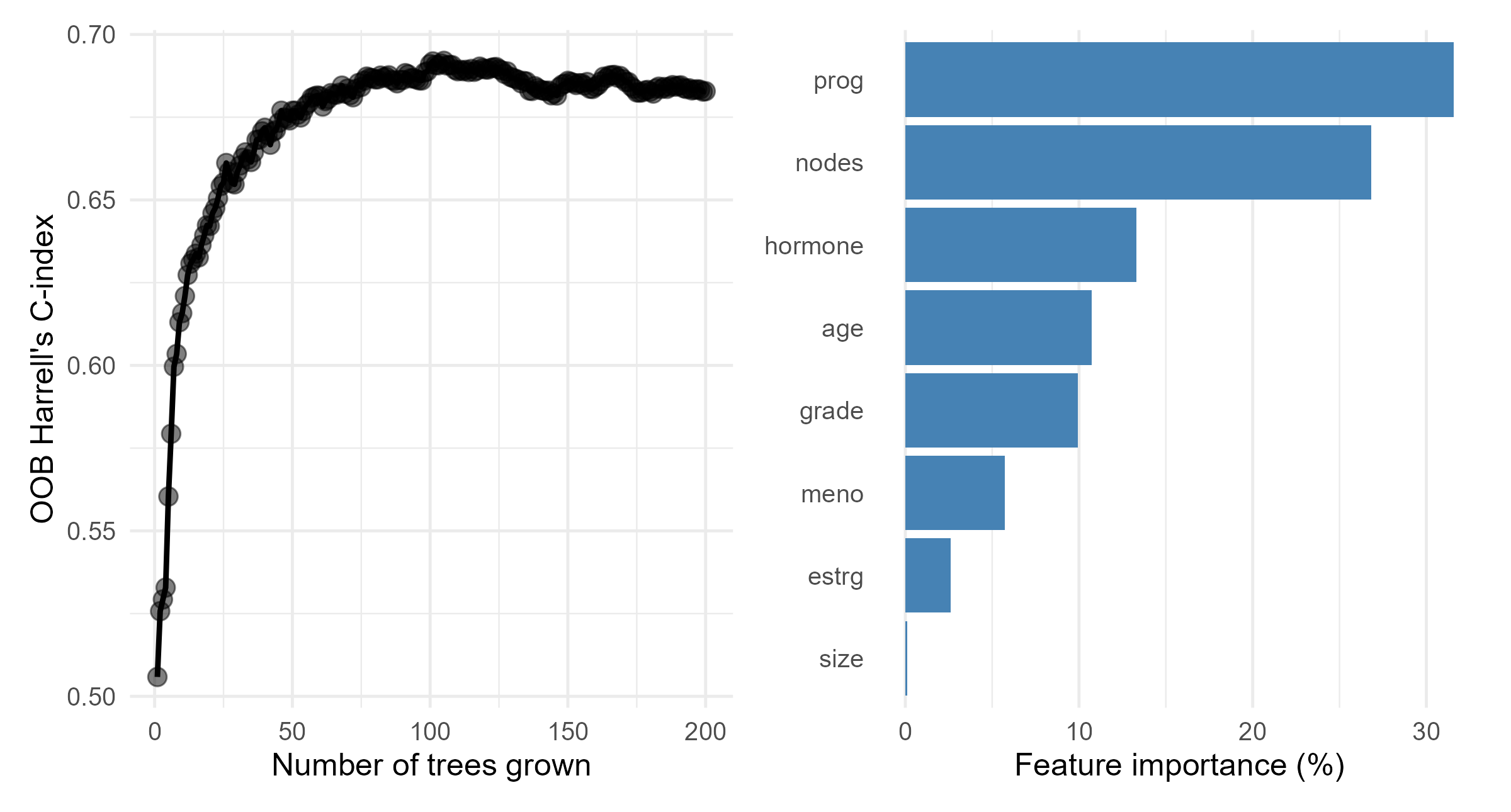
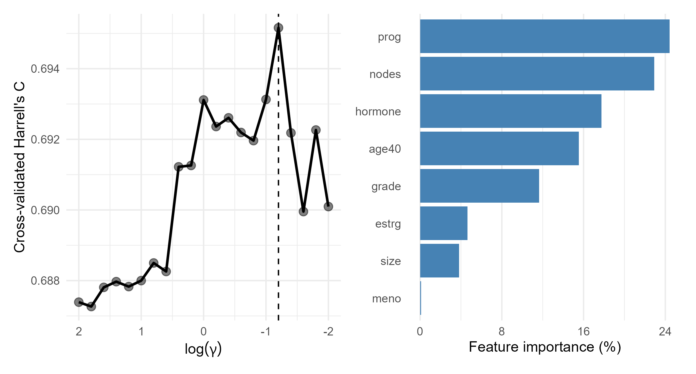
#> -----------------------------------------GBC: RSF Results
- OOB performance and variable importance
Survival Support Vector Machines
SVM for Classification
- Classification of \(Y \in \{1, -1\}\)
- Linearly separable case \[\begin{equation}\label{eq:ml:hyperplane} \left\{ \begin{aligned} \beta^\T Z_i \,+\, b &\,>\, 0 \quad \text{for all } Y_i = 1,\\[4pt] \beta^\T Z_i \,+\, b &\,<\, 0 \quad \text{for all } Y_i = -1. \end{aligned} \right. \end{equation}\]
- Hyperplane \(\beta^\T Z + b = 0\) separates two classes
- Margin: distance from hyperplane to nearest data point
- SVM: find hyperplane with maximum margin
- WLOS: normalizing coefficients and centering the hyperplane \[\begin{equation}\label{eq:ml:hyperplane_margin}
\left\{
\begin{aligned}
\beta^\T Z_i \,+\, b &\,\ge\, 1 \quad \text{for all } Y_i = 1,\\[4pt]
\beta^\T Z_i \,+\, b &\,\le\, -1 \quad \text{for all } Y_i = -1.
\end{aligned}
\right.
\end{equation}\]
- Distance between hyperplanes: \(2\|\beta\|^{-1}\)
SVM: Maximum Margin
- Maximum margin hyperplane
- Left panel: \[(\hat\beta, \hat b) \;=\; \arg\min_{\beta, b} \|\beta\|^2 \quad\text{subject to}\quad Y_i(\beta^\T Z_i + b) \ge 1,\;\; i = 1,\ldots,n\]
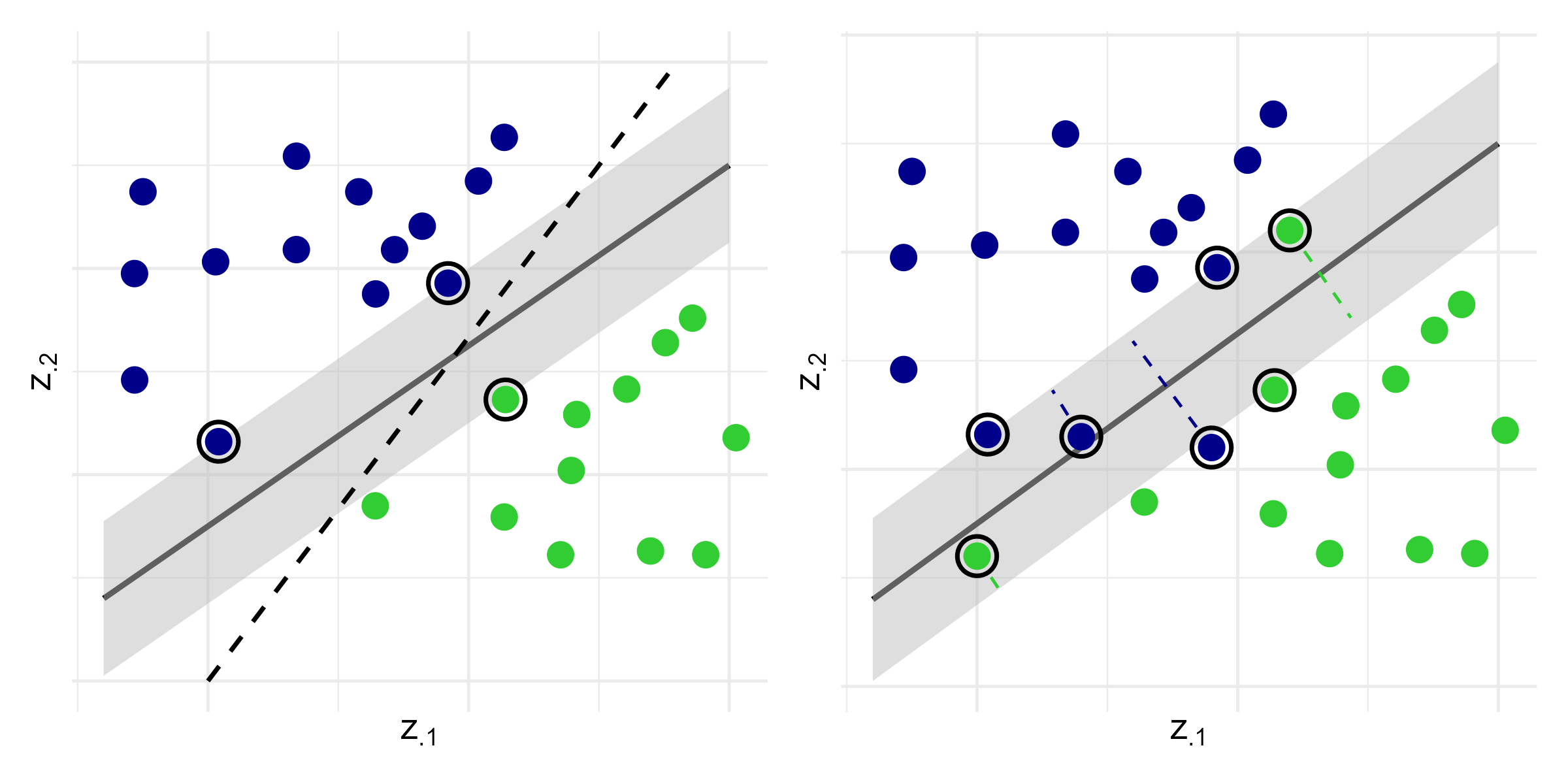
SVM: Linearly Inseparable Case
- Soft margin SVM
- Right panel: allow misclassification through slack variables \(\zeta_i \ge 0\): \[\begin{align}\label{eq:ml:svm_soft_margin} (\hat\beta, \hat b) \;=\;& \arg\min_{\beta, b,\zeta} \left\{\|\beta\|^2 \,+\, \lambda\sum_{i=1}^n\zeta_i\right\}, \notag\\ &\text{subject to}\quad \left\{ \begin{aligned} &Y_i(\beta^\T Z_i + b) \,\ge\, 1 - \zeta_i,\\[4pt] &\zeta_i \,\ge\, 0, \end{aligned} \right. \qquad i = 1,\ldots,n \end{align}\]
- Support vectors: data points with
- \(\zeta_i > 0\) (misclassified)
- \(Y_i(\hat\beta^\T Z_i + \hat b) = 1\) (on margin)
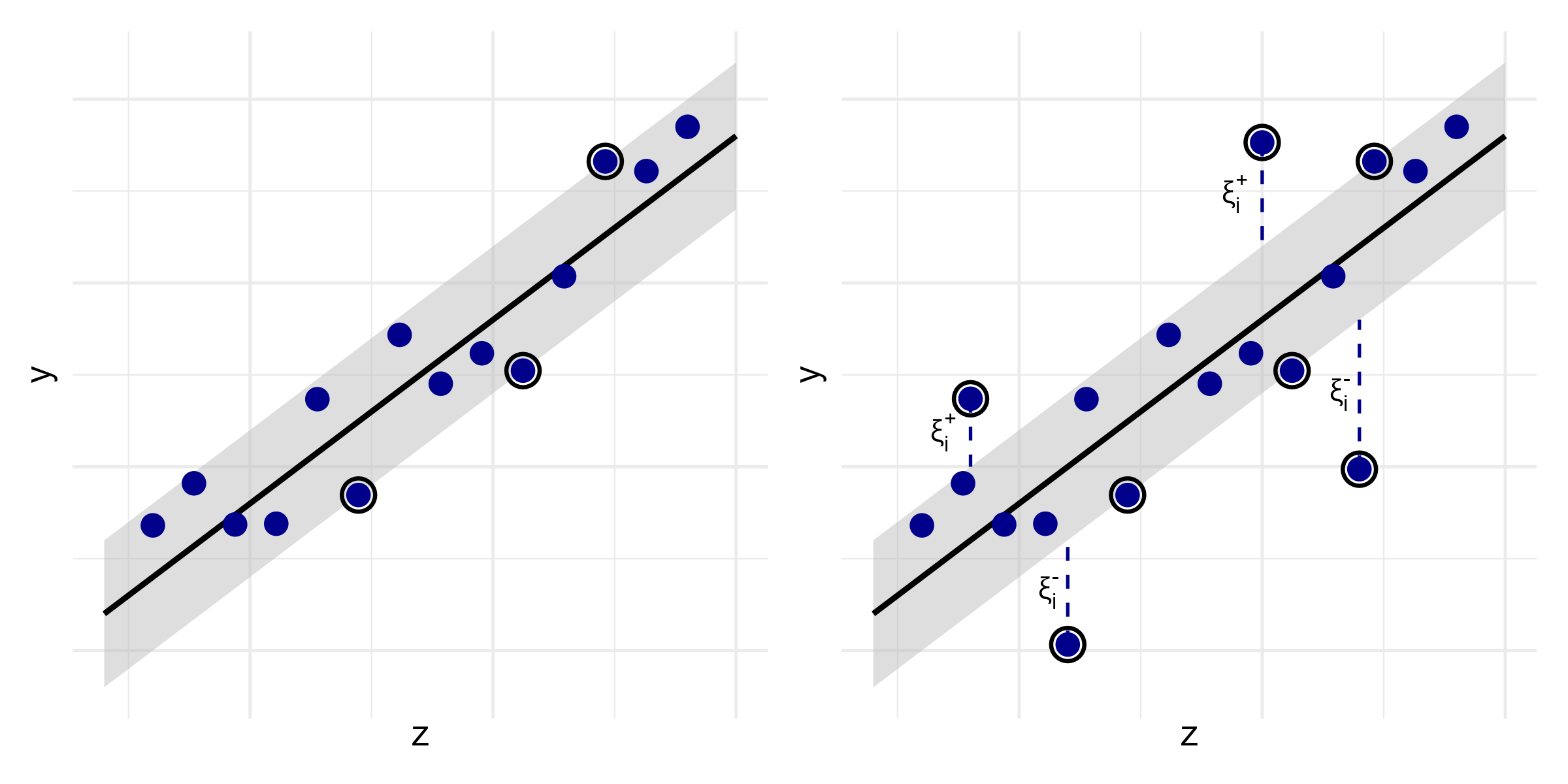
SVM: Regression (I)
- Support vector regression
- Continuous \(Y\): find hyperplane with \(\epsilon\)-insensitive loss \[\begin{equation*} (\hat\beta, \hat b) \;=\; \arg\min_{\beta, b} \|\beta\|^2 \quad\text{subject to}\quad |Y_i - (\beta^\T Z_i + b)| \,\le\, \varepsilon,\;\; i = 1,\ldots,n \end{equation*}\]
- Allow for \(\epsilon\)-insensitive slack variables \(\zeta_i^+, \zeta_i^- \ge 0\) \[\begin{align}\label{eq:ml:svm_soft_margin_reg} (\hat\beta, \hat b) \;=\;& \arg\min_{\beta, b, \xi^+, \xi^-} \left\{ \|\beta\|^2 \,+\, \lambda\sum_{i=1}^n(\xi_i^+ + \xi_i^-) \right\}, \notag\\[3pt] &\text{subject to}\quad \left\{ \begin{aligned} &Y_i - (\beta^\T Z_i + b) \,\le\, \varepsilon + \xi_i^+,\\[3pt] &(\beta^\T Z_i + b) - Y_i \,\le\, \varepsilon + \xi_i^-,\\[3pt] &\xi_i^+,\,\xi_i^- \,\ge\, 0, \end{aligned} \right. \qquad i = 1,\ldots,n \end{align}\]
SVM: Regression (II)
- Hard versus soft margin
Survival SVM (I)
- Two perspectives
- Ranking: order classification of comparable pairs \[ \mathcal P \;=\; \{(i, j):\, \delta_i = 1,\, X_i < X_j\}. \]
- Regression: predict survival time with censored data
- Ranking SSVM
- Classification with soft margin \[\begin{align}\label{eq:ml:svm_soft_margin_surv} \hat\beta \;=\;& \arg\min_{\beta, \zeta} \|\beta\|^2 \,+\, \lambda\sum_{(i, j)\in\mathcal P} \zeta_{ij}, \notag\\ &\text{subject to}\quad \left\{ \begin{aligned} &\beta^\T (Z_i - Z_j) \,\ge\, 1 - \zeta_{ij},\\[4pt] &\zeta_{ij} \,\ge\, 0, \end{aligned} \right. \qquad (i, j)\in\mathcal P \end{align}\]
Survival SVM (II)
- Regression SSVM
- Censored observations \(\to\) one-sided penalty \[\begin{align}\label{eq:ml:svm_soft_margin_reg_surv} (\hat\beta, \hat b) \;=\;& \arg\min_{\beta, b, \xi^+, \xi^-} \left\{ \|\beta\|^2 \,+\, \lambda\sum_{i=1}^n(\xi_i^+ + \xi_i^-) \right\}, \notag\\[3pt] &\text{subject to}\quad \left\{ \begin{aligned} &X_i - (\beta^\T Z_i + b) \,\le\, \xi_i^+,\\[3pt] &\delta_i\{\beta^\T Z_i + b - X_i\} \,\le\, \xi_i^-,\\[3pt] &\xi_i^+,\,\xi_i^- \,\ge\, 0, \end{aligned} \right. \qquad i = 1,\ldots,n \end{align}\]
Survival SVM (III)
- Hybrid approach
- Combines ranking and regression objective functions and penalties \[\begin{align}\label{eq:ml:svm_soft_margin_hybrid_surv} (\hat\beta, \hat b) \;=\;& \arg\min_{\beta, b, \zeta, \xi^+, \xi^-} \left\{ \|\beta\|^2 \,+\, \mu\sum_{(i,j)\in\mathcal P} \zeta_{ij} \,+\, \gamma\sum_{i=1}^n(\xi_i^+ + \xi_i^-) \right\}, \notag\\[3pt] &\text{subject to}\quad \left\{ \begin{aligned} &\beta^\T (Z_i - Z_j) \,\ge\, 1 - \zeta_{ij},\\[2pt] &\zeta_{ij} \,\ge\, 0, \end{aligned} \right. \qquad (i, j)\in\mathcal P, \notag\\[4pt] &\quad\quad\;\text{and}\quad \left\{ \begin{aligned} &X_i - (\beta^\T Z_i + b) \,\le\, \xi_i^+,\\[3pt] &\delta_i\{\beta^\T Z_i + b - X_i\} \,\le\, \xi_i^-,\\[3pt] &\xi_i^+,\,\xi_i^- \,\ge\, 0, \end{aligned} \right. \qquad i = 1,\ldots,n. \end{align}\]
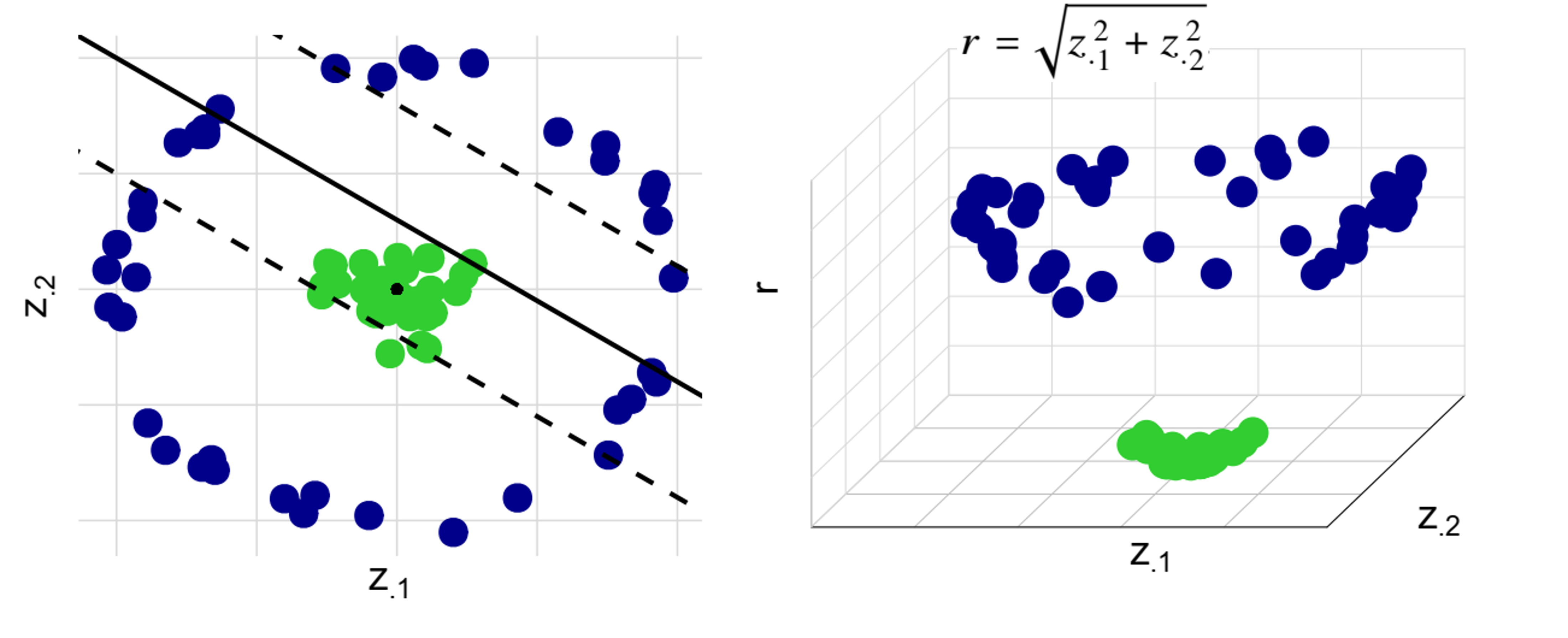
The Kernel Trick
- Nonlinear SVM
- Map covariates to high-dimensional space: \(z\mapsto \phi(z)\)
- Use kernel function \(K(z, z') = \langle \phi(z), \phi(z')\rangle\) to compute inner products
- Common kernels: linear, polynomial, radial basis function (RBF)
Software: survivalsvm::survivalsvm() (I)
- Basic syntax for fitting survival SVM
type: “ranking”, “regression”, or “hybrid”kernel: “linear”, “polynomial”, or “radial”gamma.mu: tuning parameters \(\gamma\) and \(\mu\) for hybrid SVM
Software: survivalsvm::survivalsvm() (II)
- Predict risk scores
GBC: Fitting SSVM
- Regression with linear kernel
- Feature importance computed from CV samples
GBC: Models Fitted
- Models
- Full Cox model with all predictors
- “Inadequate” Cox model excluding
progandnodes - Lasso-regularized Cox model
- Survival tree
- Random survival forest
- Survival SVM
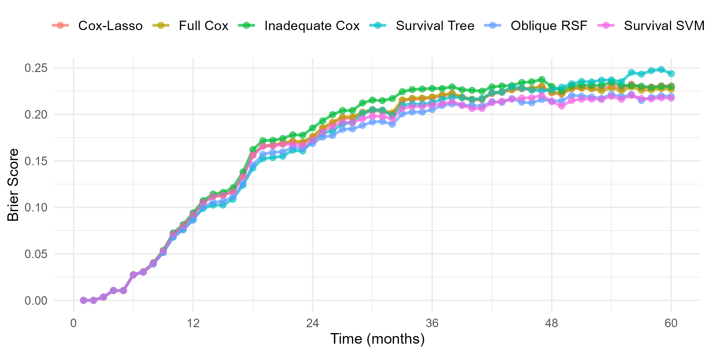
GBC: Model Evaluations
- Prediction performance on test data (\(n^*=286\))
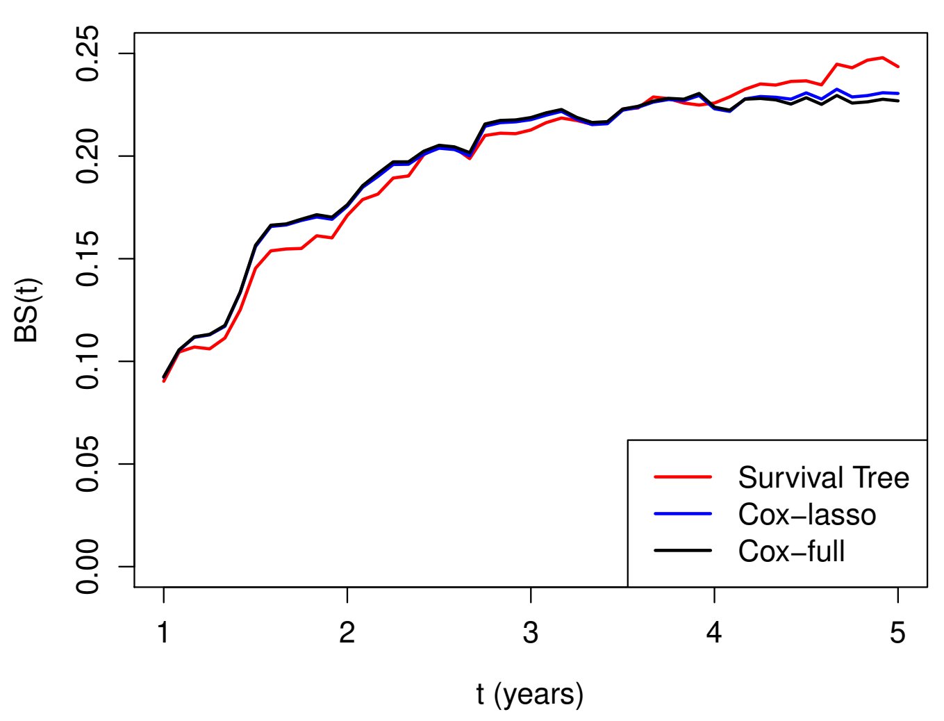
GBC: Brier Score
- Brier score over time
R’s Tidymodels System
Overview of tidymodels and censored
tidymodels: a collection of packages for modeling and machine learning in R- Provides a consistent interface for model training, tuning, and evaluation
- Key package
parsnip
- Key package
- Supports various model types, including regression, classification, and survival analysis
- Provides a consistent interface for model training, tuning, and evaluation
censored: aparsnipextension package for survival data- Implements parametric, semiparametric, and tree-based survival models
Data Preparation and Splitting
- Create a
Survobject as responseSurv(time, event)
Data splitting
initial_split(): splits data into training and testing sets
Model Specification
- Model type
survival_reg(): parametric AFT modelsproportional_hazards(penalty = tune()): (regularized) Cox PH modelsdecision_tree(cost_complexity = tune()): decision treesrand_forest(mtry = tune()): orandom forests
- Set engine and mode
set_engine("survival"): for parametric AFT modelsset_engine("glmnet"): for Cox PH modelsset_engine("aorsf"): for blique random forestsset_mode("censored regression"): for survival models
Model Specification - Example
- Example: regularized Cox model using
glmnet
Recipe and Workflow
- Recipe: a series of preprocessing steps for the data
recipe(response ~ ., data = df): specify response and predictorsstep_mutate(): standardize numeric predictorsstep_dummy(): convert categorical variables to dummy variables
- Workflow: combines model specification and recipe
workflow() |> add_model(model_spec) |> add_recipe(recipe)
Recipe and Workflow - Example
- Example: regularized Cox model with data preprocessing steps
# Create a recipe
model_recipe <- recipe(surv_obj ~ ., data = df_train) |> # specify formula
  step_mutate(z1 = z1 / 1000) |>  # standardize z1
  # group levels with prop < .02 into "other"
  step_other(z2, z3, threshold = 0.02) |>
  # convert categorical WWto dummy variables
  step_dummy(all_nominal_predictors())

# Create a workflow by combining model and recipe
model_wflow <- workflow() |>
  add_model(model_spec) |>   # add model specification
  add_recipe(model_recipe)   # add recipe
Tune Hyperparameters
- Cross-validation
df_train_folds <- vfold_cv(df_train, v = k): create k-folds on training data (default 10)tune_grid(model_wflow, resamples = df_train_folds): tuning
# k-fold cross-validation
df_train_folds <- vfold_cv(df_train, v = 10) # 10-fold cross-validation
# Tune hyperparameters
model_res <- tune_grid(
  model_wflow,
  resamples = df_train_folds,
  grid = 10, # number of hyperparameter combinations to try
  metrics = metric_set(brier_survival, brier_survival_integrated,
                       roc_auc_survival, concordance_survival), # specify metrics
  eval_time = seq(0, 84, by = 12) # evaluation time points
)
Finalize Workflow
- Examine validation results
collect_metrics(model_res): collect metrics from tuning resultsshow_best(model_res, metric = "brier_survival_integrated", n = 5): show top 5 models based on IBS
- Workflow for best model
param_best <- select_best(model_res, metric = "brier_survival_integrated"): select best hyperparameters based on Brier scorefinal_wl <- finalize_workflow(model_wflow, param_best): finalize workflow with best hyperparameters
Finalize Workflow - Example
- Example: select best hyperparameters based on Brier score and finalize workflow
Fit Final Model
- Fit the finalized workflow
final_mod <- last_fit(final_wl, split = df_split): fit the finalized workflow on the testing setcollect_metrics(final_mod): collect metrics of final model on test data
- Make predictions
predict(final_mod, new_data = new_data, type = "time"): predict survival times on new data
Fit Final Model - Example
- Example: fit the finalized workflow on the testing set, evaluate performance, and make predictions on new data
# Fit the finalized workflow on the testing set
final_mod <- last_fit(final_wl, split = df_split)

# Collect metrics of final model on test data
collect_metrics(final_mod) %>%
  filter(.metric == "brier_survival_integrated")

# Make predictions on new data
new_data <- testing(df_split) |>  slice(1:5) # take first 5 rows of test data
predict(final_mod, new_data = new_data, type = "time")
A Case Study for Tidymodels
GBC: Relapse-Free Survival
- Time to first event
library(tidymodels) # load tidymodels
library(censored)
gbc <- read.table("Data/German Breast Cancer Study/gbc.txt", header = TRUE) # Load GBC dataset
df <- gbc |>  # calculate time to first event (relapse or death)
  group_by(id) |> # group by id
  arrange(time) |> # sort rows by time
  slice(1) |>      # get the first row within each id
  ungroup() |>
  mutate(
    surv_obj = Surv(time, status), # create the Surv object as response variable
    .after = id, # keep id column after surv_obj
    .keep = "unused" # discard original time and status columns
  )
Data Preparation
- Analysis dataset
# A tibble: 6 × 10
     id   surv_obj hormone   age  meno  size grade nodes  prog estrg
  <int>     <Surv>   <int> <int> <int> <int> <int> <int> <int> <int>
1     1 43.836066        1    38     1    18     3     5   141   105
2     2 46.557377        1    52     1    20     1     1    78    14
3     3 41.934426        1    47     1    30     2     1   422    89
4     4  4.852459+       1    40     1    24     1     3    25    11
5     5 61.081967+       2    64     2    19     2     1    19     9
6 6 63.377049+ 2 49 2 56 1 3 356 64Models to be Trained
- Regularized Cox model
proportional_hazards(penalty = tune())(Default: \(\alpha = 1\); lasso)- Tune penalty parameter \(\lambda\)
- Use
glmnetengine for fitting
- Random forest
rand_forest(mtry = tune(), min_n = tune())- Tune number of predictors to split on and minimum size of terminal node
- Use
aorsfengine for fitting
Common Recipe
- Recipe for both models
gbc_recipe <- recipe(surv_obj ~ ., data = gbc_train) |> # specify formula
  step_mutate(
    grade = factor(grade),
    age40 = as.numeric(age >= 40), # create a binary variable for age >= 40
    prog = prog / 100, # rescale prog
    estrg = estrg / 100 # rescale estrg
  ) |>
  step_dummy(grade) |>
  step_rm(id) # remove id
# gbc_recipe # print recipe information
Regularized Cox Model
- Cox model specification and workflow
# Regularized Cox model specification
cox_spec <- proportional_hazards(penalty = tune()) |>  # tune lambda
  set_engine("glmnet") |>  # set engine to glmnet
  set_mode("censored regression") # set mode to censored regression
cox_spec # print model specification
Proportional Hazards Model Specification (censored regression)
Main Arguments:
penalty = tune()
Computational engine: glmnet Model Tuning
- Cross-validation set-up
set.seed(123) # set seed for reproducibility
gbc_folds <- vfold_cv(gbc_train, v = 10) # 10-fold cross-validation
# Set evaulation metrics
gbc_metrics <- metric_set(brier_survival, brier_survival_integrated,
                          roc_auc_survival, concordance_survival)
gbc_metrics # evaluation metrics info
A metric set, consisting of:
- `brier_survival()`, a dynamic survival metric | direction:
minimize
- `brier_survival_integrated()`, a integrated survival metric | direction:
minimize
- `roc_auc_survival()`, a dynamic survival metric | direction:
maximize
- `concordance_survival()`, a static survival metric | direction:
maximizeCox Model Tuning
- Tune the regularized Cox model
- Use
tune_grid()to perform hyperparameter tuning - Evaluate performance using Brier score and ROC AUC
- Use
set.seed(123) # set seed for reproducibility
# Tune the regularized Cox model (this will take some time)
cox_res <- tune_grid(
  cox_wflow,
  resamples = gbc_folds,
  grid = 10, # number of hyperparameter combinations to try
  metrics = gbc_metrics, # evaluation metrics
  eval_time = time_points, # evaluation time points
  control = control_grid(save_workflow = TRUE) # save workflow
)
Cox Model Tuning Results
- Plot IBS as function of \(\log\lambda\)
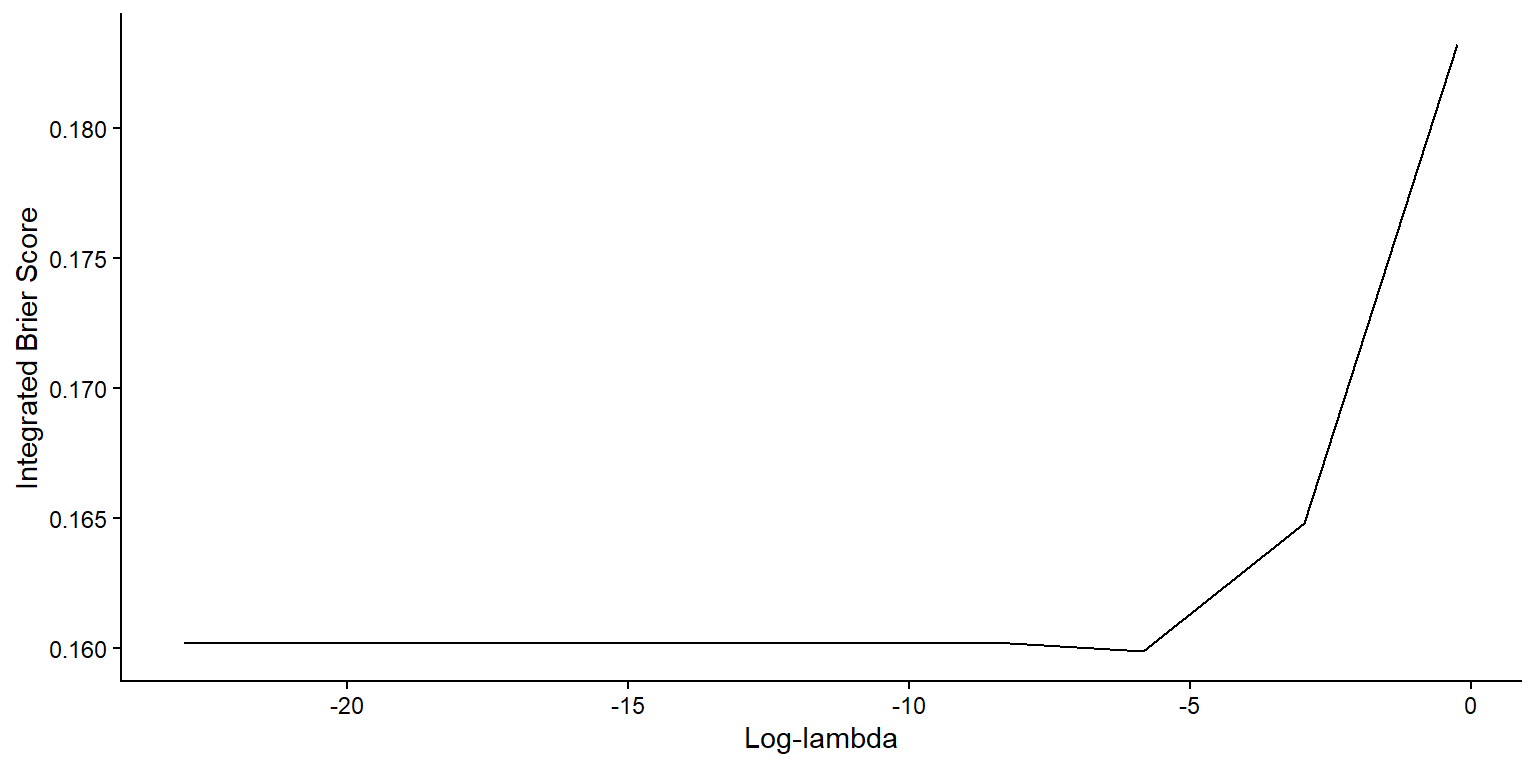
Best Cox Models
- Show best models
- Based on Brier score
# A tibble: 5 × 8
   penalty .metric             .estimator .eval_time  mean     n std_err .config
     <dbl> <chr>               <chr>           <dbl> <dbl> <int>   <dbl> <chr>
1 2.92e- 3 brier_survival_int… standard           NA 0.160    10 0.00765 pre0_m…
2 1.15e-10 brier_survival_int… standard           NA 0.160    10 0.00775 pre0_m…
3 1.44e- 9 brier_survival_int… standard           NA 0.160    10 0.00775 pre0_m…
4 1.30e- 8 brier_survival_int… standard           NA 0.160    10 0.00775 pre0_m…
5 1.17e- 7 brier_survival_int… standard           NA 0.160    10 0.00775 pre0_m…
Random Forest Model
- Random forest specification and workflow
# Random forest model specification
rf_spec <- rand_forest(mtry = tune(), min_n = tune()) |>  # tune mtry and min_n
  set_engine("aorsf") |>  # set engine to aorsf
  set_mode("censored regression") # set mode to censored regression
rf_spec # print model specification
Random Forest Model Specification (censored regression)
Main Arguments:
mtry = tune()
min_n = tune()
Computational engine: aorsf Random Forest Tuning
- Tune the random forest model
- Similar to Cox model tuning
set.seed(123) # set seed for reproducibility
# Tune the random forest model (this will take some time)
rf_res <- tune_grid(
  rf_wflow,
  resamples = gbc_folds,
  grid = 10, # number of hyperparameter combinations to try
  metrics = gbc_metrics, # evaluation metrics
  eval_time = time_points # evaluation time points
)
Random Forest Tuning Results
- View validation results
# A tibble: 6 × 9
   mtry min_n .metric         .estimator .eval_time   mean     n std_err .config
  <int> <int> <chr>           <chr>           <dbl>  <dbl> <int>   <dbl> <chr>
1     1    14 brier_survival  standard            0 0         10 0       pre0_m…
2     1    14 roc_auc_surviv… standard            0 0.5       10 0       pre0_m…
3     1    14 brier_survival  standard           12 0.0643    10 0.00748 pre0_m…
4     1    14 roc_auc_surviv… standard           12 0.838     10 0.0312  pre0_m…
5     1    14 brier_survival  standard           24 0.165     10 0.0103  pre0_m…
6     1    14 roc_auc_surviv… standard           24 0.753     10 0.0470  pre0_m…
Best Random Forest Models
- Show best models
- Based on Brier score
# A tibble: 5 × 9
   mtry min_n .metric          .estimator .eval_time  mean     n std_err .config
  <int> <int> <chr>            <chr>           <dbl> <dbl> <int>   <dbl> <chr>
1     5    35 brier_survival_… standard           NA 0.155    10 0.00775 pre0_m…
2     8    40 brier_survival_… standard           NA 0.155    10 0.00745 pre0_m…
3     7    23 brier_survival_… standard           NA 0.155    10 0.00758 pre0_m…
4    10    27 brier_survival_… standard           NA 0.156    10 0.00731 pre0_m…
5 4 18 brier_survival_… standard NA 0.156 10 0.00795 pre0_m…- Conclusion
- Best RF model has lower Brier score than best Cox model
Finalize and Fit Best Model
- Fit final RF model
# Select best RF hyperparameters (mtry, min_n) based on Brier score
param_best <- select_best(rf_res, metric = "brier_survival_integrated")
param_best # view results
# A tibble: 1 × 3
mtry min_n .config
<int> <int> <chr>
1 5 35 pre0_mod05_post0rf_final_wflow <- finalize_workflow(rf_wflow, param_best) # Finalize workflow
# Fit the finalized workflow on the testing set
set.seed(123) # set seed for reproducibility
final_rf_fit <- last_fit(
rf_final_wflow,
split = gbc_split, # use the original split
metrics = gbc_metrics, # evaluation metrics
eval_time = time_points # evaluation time points
)Test Performance (I)
- Collect metrics on test data
collect_metrics(final_rf_fit) |> # collect overall performance metrics
  filter(.metric %in% c("concordance_survival", "brier_survival_integrated"))
# A tibble: 2 × 5
.metric .estimator .eval_time .estimate .config
<chr> <chr> <dbl> <dbl> <chr>
1 brier_survival_integrated standard NA 0.235 pre0_mod0_post0
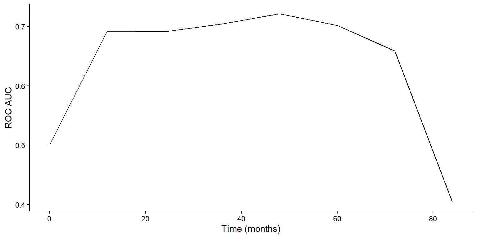
2 concordance_survival standard NA 0.655 pre0_mod0_post0Test Performance (II)
- Plot test ROC AUC over time
Prediction by Final RF Model
- Extract the fitted workflow
- Use
extract_workflow()to get the final model
- Use
gbc_rf <- extract_workflow(final_rf_fit) # extract the fitted workflow
# Predict on new data
gbc_5 <- testing(gbc_split) |>  slice(1:5) # take first 5 rows of test data
predict(gbc_rf, new_data = gbc_5, type = "time") # predict survival times
# A tibble: 5 × 1
.pred_time
<dbl>
1 48.2
2 66.4
3 66.2
4 36.6
5 49.7Survival Tree Exercise
- Task: fit a survival tree model to the GBC data
- Use
decision_tree()withset_engine("rpart") - Tune complexity parameter
cost_complexityusingtune() - Use the same recipe as for Cox and RF models
- Evaluate performance using Brier score and ROC AUC
- Use
Conclusion
Notes (I)
- The lasso
- First proposed by Tibshirani (1996) for least-squares
- Extended to Cox model by Tibshirani (1997)
- Algorithms for \(L_1\)-regularized Cox model described in Simon et al. (2011)
- Variations
- group lasso (Yuan and Lin, 2006)
- adaptive lasso (Zou, 2006)
- smoothly clipped absolute deviations (SCAD; Xie and Huang, 2009)
- Elastic net for win ratio
- WRnet (Mao, 2025)
Notes (II)
- More on decision trees
- Text: Breiman et al. (1984)
- Review article: Bou-Hamad et al. (2011, Statistics Surveys)
- Bagging and random forests (R-packages)
ipredrandomSurvivalForestranger

Notes (III)
- Python’s machine learning systems
scikit-learn: general machine learning library with support for survival analysis through extensions likescikit-survivallifelines: library specifically for survival analysis, including Cox models and KM estimatorsxgboostandlightgbm: gradient boosting libraries adaptable for survival analysis using custom loss functions
- Deep learning in survival analysis
DeepSurv: a deep learning-based Cox proportional hazards modelDeepHit: a deep learning model for competing risks survival analysis
Summary (I)
- Regularized Cox model
- Elastic net \[
Q_n(\beta;\lambda) = \ell_n(\beta) - \lambda\left\{\alpha\|\beta\|_1 + (1-\alpha)\|\beta\|_2^2/2\right\}
\]
glmnet::glmnet(Z, Surv(time, status), family = “cox”, alpha = 1)
- Elastic net \[
Q_n(\beta;\lambda) = \ell_n(\beta) - \lambda\left\{\alpha\|\beta\|_1 + (1-\alpha)\|\beta\|_2^2/2\right\}
\]
- Survival trees
- Root node \(\to\) recursive partitioning based on similarity in outcome \(\to\) pruning to prevent overfitting
rpart:: rpart(Surv(time, status) ~ covariates)
- Root node \(\to\) recursive partitioning based on similarity in outcome \(\to\) pruning to prevent overfitting
Summary (II)
- Random survival forests
- Ensemble of survival trees with random feature selection and bootstrap
aorsf:: aorsf(Surv(time, status) ~ covariates, n_tree = 200)
- Ensemble of survival trees with random feature selection and bootstrap
- Survival SVM
- Extension of SVM for survival data using ranking or regression approaches
- R’s
tidymodelssystem- A consistent interface for model training, tuning, and evaluation
censoredpackage extendsparsnipfor survival models