Applied Survival Analysis

Chapter 14 - Causal Inference in Survival Analysis

Lu Mao

lmao@biostat.wisc.edu

Department of Biostatistics & Medical Informatics

University of Wisconsin-Madison

Outline

The counterfactual framework
Inverse weighting and standardization
Estimating causal survival curves
Marginal structural models with time-varying treatment/confounding

\[\newcommand{\d}{{\rm d}}\] \[\newcommand{\T}{{\rm T}}\] \[\newcommand{\dd}{{\rm d}}\] \[\newcommand{\cc}{{\rm c}}\] \[\newcommand{\pr}{{\rm pr}}\] \[\newcommand{\var}{{\rm var}}\] \[\newcommand{\se}{{\rm se}}\] \[\newcommand{\indep}{\perp \!\!\! \perp}\] \[\newcommand{\Pn}{n^{-1}\sum_{i=1}^n}\] \[ \newcommand\mymathop[1]{\mathop{\operatorname{#1}}} \] \[ \newcommand{\Ut}{{n \choose 2}^{-1}\sum_{i<j}\sum} \]

The Counterfactual Framework

Association vs Causation

Statistical inference
- Association: test of group difference, correlation, regression
- Causation: informal or irrelevant
Causal inference: study causal relationships explicitly
- Counterfactual framework
- Causal diagrams
Motivating example: German Breast Cancer Study
- Relapse-free survival ($T$) vs hormonal therapy ($A=1$ yes; $A=0$: no)
- First assume $T$ is fully observed (no censoring)

RCT as Gold Standard

Randomized controlled trial (RCT)
- Patients randomly assigned to hormonal vs non-hormonal treatment
- Two groups identical (exchangeable) in terms of baseline characteristic
- Any between-group difference in relapse-free survival attributable to treatment (no confounding)
  - Increase in $t=5$ years relapse-free survival rate caused by hormonal treatment
  \[ \hat\pr(T>t\mid A=1)-\hat\pr(T>t\mid A=0) \]
  - (Causal) Hazard ratio under Cox model with binary group as covariate

Possible Confounding

Hormone non-randomized
- Women under hormonal treatment more likely to be post-menopausal than non-treatment (76.0% vs 47.5%)
- Difference in RFS $\to$ treatment or menopause?
- Confounder: menopausal status

Traditional Methods

Adjustment for confounding
- Log-rank test stratified by menopausal status (Ch. 3; stratum-specific difference)
- Cox regression with menopausal status as a covariate (Ch. 4; conditional hazard ratio)
- Neither provides a population-level causal effect size of hormone treatment like that derived from an RCT
Goal
- Drawing causal inference in an RCT-like setting, even with observational data

Counterfactual Framework

Potential outcomes
- Each subject has two potential outcomes $T^{(a)}$ $(a=1, 0)$
  - $T^{(1)}$: had the subject been assigned to treatment
  - $T^{(0)}$: had the subject been assigned to control
Causal estimand
- Any contrast in distribution between $T^{(1)}$ vs $T^{(0)}$
- Example
  - Survival probability: $\pr(T^{(1)}>t)-\pr(T^{(0)}>t)$
  - RMST: $E(T^{(1)}\wedge t) - E(T^{(0)}\wedge t)$

Exchangeability Assumption

Observed outcome
- $A = 1, 0$: actually assigned group \[T=AT^{(1)}+(1-A)T^{(0)}\,\,\,\, (\rm consistency)\]
Assumptions
- Complete randomization $T^{(a)}\indep A,\hspace{5mm}a=1, 0$
  - Too strong, typically not satisfied
- Conditional exchangeability \[\begin{equation}\label{eq:causal:cond_exch} T^{(a)}\indep A \mid W,\hspace{5mm} a=1, 0 \end{equation}\]
  - Assignment independent of potential outcome given confounders $W$
  - All confounders are captured in $W$

Causal Diagrams

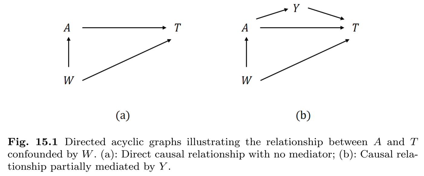
Directed Acyclic Graph

IPTW & Standardization

Estimand

Observed data
- Assume the $T_i$ are fully observed \[(T_i, A_i, W_i),\,\,\,\, i=1,\ldots, n\]
Two classes of methods
- Inverse probability treatment weighting (IPTW)
- Standardization
Causal estimand \[\begin{equation*} S_a(t)=\pr(T^{(a)}>t) \end{equation*}\]

Propensity Score

Selection bias
- $(Y\mid A = 1)$ and $(Y\mid A = 0)$ non-representative of general population
- Naive estimator biased \[ \hat S_a^{\rm naive}(t)=\frac{\sum_{i=1}^nI(A_i=a, T_i>t)}{\sum_{i=1}^nI(A_i = a)} \]
Propensity score
- Probability of entering treatment $a$ \[\begin{equation} \pi_a(W)=\pr(A=a\mid W) \end{equation}\]
- General population $\stackrel{\pi_a(W)}{\rightleftarrows}$ Group $a$

IPTW

Re-constitute general population
- Inverse weighting: Group $a$ $\stackrel{\pi_a(W)^{-1}}{\rightarrow}$ General population \[\begin{equation}\label{eq:causal:ipw_surv} \hat S_a^{\rm IP}(t)=n^{-1}\sum_{i=1}^n\frac{I(A_i=a, T_i>t)}{\pi_a(W_i)} \end{equation}\]
- Unbiased \[\begin{align*} E\left\{\frac{I(A=a, T>t)}{\pi_a(W)}\right\}&=E\left\{\frac{I(A=a, T^{(a)}>t)}{\pi_a(W)}\right\}\\ &=E\left[\pi_a(W)^{-1}E\left\{I(A=a, T^{(a)}>t)\mid W\right\}\right]\\ &=E\left\{\pi_a(W)^{-1}\pr(A=a\mid W)\pr(T^{(a)}>t\mid W)\right\}\\ &=E\left\{\pr(T^{(a)}>t\mid W)\right\}\\ &=S_a(t) \end{align*}\]

Estimate Propensity Score

$\pi_a(W)$ unknown unless by design
- Estimate $\hat\pi_a(\cdot)$ using \[ (A_i, W_i),\,\,\ i=1,\ldots,n \]
- Logistic regression
- Machine learning classification
IPTW estimator
- Plug in $\hat\pi_a(W_i)$ \[\begin{equation} \hat S_a^{\rm IP}(t)=n^{-1}\sum_{i=1}^n\frac{I(A_i=a, T_i>t)}{\hat\pi_a(W_i)} \end{equation}\]
- Variance estimation needs to account for randomness in $\hat\pi_a(\cdot)$

Standardization

Model outcome vs confounder
- Instead of treatment vs confounder \[ \hat S_a(t\mid W)= \hat\pr(T^{(a)}>t\mid W) \]
- E.g., Cox model based on \[ \{(T_i, W_i): A_i=a, i=1,\ldots, n\} \]
- $(T\mid A =a, W) = (T^{(a)}\mid A =a, W) = (T^{(a)}\mid W)$ (conditional exchangeability)
Standardized estimator
- Average across population: $\hat S_a^{\rm reg}(t)=n^{-1}\sum_{i=1}^n\hat S_a(t\mid W_i)$

IPTW vs Standardization

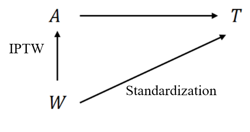
Modeling target
- IPTW: treatment vs confounder
- Standardization: outcome vs confounder
Properties
- Nonparametric setting (categorical confounder): $\hat S_a^{\rm IP}(t)=\hat S_a^{\rm reg}(t)$
- Doubly robust estimator: valid when either model is true, efficient when both are true

Estimating Causal Survival Curves

Dealing with Censored Data

In presence of censoring
- IPTW (+ IPCW)
- Standardardization (adjust for cenosring)
Observed data \[ (X, \delta, A, W) \]
- $X=T\wedge C$, $\delta = I(T\leq C)$, $C$: censoring time
Two levels of coarsening
- $T^{(a)}\to T$: treatment assignment
- $T\to (X, \delta)$: Censoring

Assumptions about Censoring

Two types of assumption
- Censoring depends on confounder (general) \[\begin{equation}\label{eq:causal:indep_cens1} T\indep C\mid (A, W) \end{equation}\]
- Censoring not dependent on confounder \[\begin{equation}\label{eq:causal:indep_cens2} T\indep C\mid A \end{equation}\]

IPCW

General assumption $(W\to C)$
- Adjust for selection bias by censoring
- Inverse probability treatment weighting (IPTW) + Inverse probability censoring weighting (IPCW)
Censoring weight
- $G_a(t\mid W)=\pr(C\geq t\mid A=a, W)$
- E.g., Cox model fit on \[ (X_i, 1-\delta_i, W_i)\,\,\,\, i=1,\ldots, n \] with $C_i$ as outcome

Inverse Weighting

Selection probability
- In group $a$ and not censored by $t$: $\pi_a(W)G_a(t\mid W)$
- Inverse weight \[ \hat w_{ai}(t)=\frac{I(A_i=a)}{\hat\pi_a(W_i)\hat G_a(t\mid W_i)} \]
IPT(C)W-adjusted KM estimator
- $N_i(t)=I(X_i\leq t,\delta_i=1)$ \[\begin{equation}\label{eq:causal_ipcw} \hat S_a^{\rm IP}(t)=\prod_{0\leq u\leq t}\left\{1-\frac{\sum_{i=1}^n \hat w_{ai}(u)\dd N_i(u)}{\sum_{i=1}^n \hat w_{ai}(u)I(X_i\geq u)}\right\} \end{equation}\]
- If $(T\indep C)\mid A$, then $\hat G_a(t\mid W_i)\equiv 1$

Causal Cox Model

Marginal structural model
- $\lambda_a(t)$: hazard function of $T^{(a)}$ \[\begin{equation}\label{eq:causal:msm_cox} \lambda_a(t)=\exp(a\beta)\lambda_0(t) \end{equation}\]
IPT(C)W-adjusted partial likelihood score
- $\hat w_i(t)=\{\hat\pi_{A_i}(W_i)\hat G_{A_i}(t\mid W_i)\}^{-1}$ \[\begin{equation}\label{eq:causal:score} n^{-1}\sum_{i=1}^n\int_0^\infty\left\{A_i-\frac{\sum_{j=1}^nA_j\hat w_{j}(t) I(X_j\geq t)\exp(A_j\beta)} {\sum_{j=1}^n \hat w_{j}(t) I(X_j\geq t)\exp(A_j\beta)}\right\}\hat w_{i}(t)\dd N_i(t)=0 \end{equation}\]
- $\exp(\beta)$: causal hazard ratio

Standardization Approach

Two-steps
- Outcome (censored) vs confounder \[S_a(t\mid W)=\pr(T^{(a)}>t\mid W)\]
- Average $\hat S_a^{\rm reg}(t)=n^{-1}\sum_{i=1}^n\hat S_a(t\mid W_i)$
- Standard software

Software: `ipw::ipwpoint()`

Basic syntax for computing propensity scores
- A: A; confounders: W
- family = "binomial", link="logit": logistic regression for binary $A$

tmp <- ipwpoint(exposure = A, denominator=~ confounders,
                family = "binomial", link="logit")

Output

tmp$ipw.weights: $n$-Vector of inverse weights
Plug in survfit() and coxph()

# IPTW-adjusted KM
obj <- survfit(Surv(time,status) ~ A, weights = tmp$ipw.weights)

GBC: An Example

German Breast Cancer study
- $A$: hormone treatment (1) vs no treatment (0)
- $T$: relapse-free survival time
- $𝑊$: confounders (menopausal status, tumor size, tumor grade, progesterone and estrogen receptor levels)
Assumption about censoring
- For simplicity \[(T\indep C)\mid A\] Only IPTW needed (no IPCW)

GBC: Coding & Results

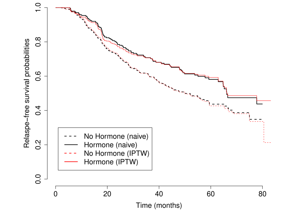
IPTW-adjusted vs unweighted KM
- Causal hazard ratio: 69.5% ($p$-value 0.006)
- Standard error may be incorrect due to randomness in estimated weights
  - Bootstrap

# estimate propensity score
tmp <- ipwpoint(exposure = A, family="binomial",link="logit",
             denominator =~ meno + size + factor(grade) + nodes + prog 
                      + estrg, data=data.CE)
# IPTW-adjusted KM
obj <- survfit(Surv(time, status) ~ A, weights = tmp$ipw.weights, 
                       data = data.CE)
# IPTW Cox model (essentially a marginal structural Cox model)
coxph(Surv(time,status) ~ A, weights=tmp$ipw.weights, data=data.CE)
#>       coef exp(coef) se(coef) robust se     z       p
#> A -0.36947   0.69110  0.08318   0.13632 -2.71 0.00672

GBC: IPTW vs Naive

Confounding not obvious

Marginal Structural Models (MSM)

Point Treatment

Causal inference
- Relationship between $T^{(a)}$ vs $a$, rather than $T$ vs $A$
Marginal structural models
- Definition: a model for $T^{(a)}$ against $a$, possibly adjusting for baseline covariates $v\subset W$
- Marginal: no need to condition on full $W$ as covariates
- Structural: treatment is $a$ (as in RCT), not observed $A$
- Simplest case: $V=\emptyset$ \[\begin{equation} \lambda_a(t)=\exp(a\beta)\lambda_0(t) \end{equation}\]
- Concept most useful in time-varying treatment/confounding

Marginal Structural Cox Model

General form
- $\lambda_a(t\mid V)$: conditional hazard of $T^{(a)}$ given $V$ \[\begin{equation}\label{eq:causal:msm_cox1} \lambda_a(t\mid V)=\exp(\beta a+\gamma^{\rm T}V)\lambda_0(t) \end{equation}\]
- $\exp(\beta)$: causal hazard ratio for treatment vs control adjusting for $V$
  - Different from the causal HR adjusting for all of $W$
- Treatment $\times$ covariate interaction \[\begin{equation}\label{eq:causal:msm_cox2} \lambda_a(t\mid V)=\exp(\beta a+\gamma^{\rm T}V+a\eta^{\rm T}V)\lambda_0(t) \end{equation}\]

Fitting MSM

General assumption: $T\indep C\mid (A, W)$
Weight construction
- Standard IPTW-IPCW weights \[w_i(t)=\frac{1}{\pi_{A_i}(W_i)G_{A_i}(t\mid W_i)}\]
- Stablized IPTW-IPCW weights \[\begin{equation}\label{eq:causal:swights} w^{\rm s}_i(t)=\frac{\pi_{A_i}(V_i)G_{A_i}(t\mid V_i)}{\pi_{A_i}(W_i)G_{A_i}(t\mid W_i)}, \end{equation}\]
  - $\pi_{a}(V)=\pr(A=a\mid V)$ and $G_{a}(t\mid V)=\pr(C>t\mid A=a, V)$
  - Set $G_{a}(t\mid V)=G_{a}(t\mid W)\equiv 1$ if $W\not\to C$

Weighted Partial-Likelihood Score

Using stablized weights
- $\hat w^{\rm s}_i(t)$: an estimate of $w^{\rm s}_i(t)$ \[\begin{equation}\label{eq:causal:msm_ee} n^{-1}\sum_{i=1}^n\int_0^\infty\left\{Z_i-\frac{\sum_{j=1}^nZ_j\hat w^{\rm s}_j(t) I(X_j\geq t)\exp(\zeta^{\rm T}Z_j)} {\sum_{j=1}^n \hat w^{\rm s}_j(t) I(X_j\geq t)\exp(\zeta^{\rm T}Z_j)}\right\} \hat w^{\rm s}_i(t)\dd N_i(t)=0 \end{equation}\]
- $Z_i=(A_i, V_i^{\rm T})^{\rm T}$ and $\zeta=(\beta,\gamma^{\rm T})^{\rm T}$

Time-Varying Treatment

MSM
- Adjust for confounders $\not\leftrightarrow$ adjust for covariates
- Conditioning on covariate changes meaning of covariate effects
Most useful in time-varying treatment/confounding
- Mediator of previous treatment $\leftrightarrow$ Confounder for current/future treatment
- Previous anti-retroviral treatment $\to$ current CD4 count $\stackrel{\rm prescribe}{\rightarrow}$
  - Conditioning on CD4 $\to$ corrects confounding for current trt, blocks causal path of previous trt

Notation & DAG

Notation
- $a(t)$: hypothetical treatment at $t$; $A(t)$: observed treatment at $t$
- $W(t)$: possible confounders at $t$
- Discretization
  - $0=t_0<t_1<\cdots<t_m$: time points
  - $A_{\cdot j}=A(t_j)$ and $W_{\cdot j}=W(t_j)$
  - $\overline A_{\cdot j}=\{A_{\cdot 0},\ldots, A_{\cdot j}\}$; $\overline W_{\cdot j}=\{W_{\cdot 0},\ldots, W_{\cdot j}\}$; $V\subset W_{\cdot 0}$: baseline covariates

MSM for Time-Varying Treatment

Modeling target
- Treatment path (sequence): $\overline a(t)=\{a(u): 0\leq u\leq t\}$
- Outcome: $T^{(\overline a)}$ = potential outcome under treatment path $\overline a(\infty)$ against $a(\cdot)$
Model specification
- $\lambda_{\overline a}(t\mid V)$: conditional hazard of $T^{(\overline a)}$ given $V$ \[\begin{equation}\label{eq:causal:msm_tv} \lambda_{\overline a}(t\mid V)=\exp\{\beta a(t)+\gamma^{\rm T}V\} \end{equation}\]
- Cox model with external (why?) time-varying covariate $a(t)$
  - Replace $a(t)$ by any summary of $\overline a(t)$, e.g., total time on treatment

Sequential Randomization Assumption

Sequential conditional exchangeability
- An time-varying version of CE \[\begin{equation}\label{eq:causal:cond_exch1} T^{(\overline a)}\indep A_{\cdot j}\mid (\overline A_{\cdot, j-1}, \overline W_{\cdot j}) \hspace{2mm}j=1,\ldots, m. \end{equation}\]
- Treatment assignment random given previous treatments and current/previous confounders (biomarkers)

Longitudinal Weights

At time $t_j$
- Propensity scores/non-censoring hazards \[\begin{align} \pi_k(t_j; \overline A_{\cdot, j-1}, V)&=\pr(A_{\cdot j}=k\mid \overline A_{\cdot, j-1}, V)\\ \pi_k(t_j; \overline A_{\cdot, j-1}, \overline W_{\cdot j})&=\pr(A_{\cdot j}=k\mid \overline A_{\cdot, j-1}, \overline W_{\cdot j})\\ \lambda_C(t_j\mid \overline A_{\cdot, j-1}, V)&=\pr(C>t_j \mid C>t_{j-1}, \overline A_{\cdot, j-1}, V)\\ \lambda_C(t_j\mid \overline A_{\cdot, j-1}, \overline W_{\cdot j})&=\pr(C>t_j \mid C>t_{j-1}, \overline A_{\cdot, j-1}, \overline W_{\cdot j}) \end{align}\]
Stablized weight at $t$
- IPTW + IPCW \[\begin{equation}\label{eq:causal:swights_tv} w^{\rm s}(t)=\prod_{t_j\leq t}\frac{\pi_{A_{\cdot, j}}(t_j; \overline A_{\cdot, j-1}, V)\lambda_C(t_j\mid \overline A_{\cdot, j-1}, V)} {\pi_{A_{\cdot, j}}(t_j; \overline A_{\cdot, j-1}, \overline W_{\cdot j})\lambda_C(t_j\mid \overline A_{\cdot, j-1}, \overline W_{\cdot j})} \end{equation}\]

Weighted Partial-Likelihood Score

Using stablized weights
- $\hat w^{\rm s}_i(t)$: estimated $w^{\rm s}(t)$ for $i$th subject \[\begin{align*} n^{-1}\sum_{i=1}^n\int_0^\infty\left\{Z_i(t)-\frac{\sum_{j=1}^n\hat w^{\rm s}_j(t) Z_j(t) I(X_j\geq t)\exp\{\zeta^{\rm T}Z_j(t)\}} {\sum_{j=1}^n \hat w^{\rm s}_j(t) I(X_j\geq t)\exp\{\zeta^{\rm T}Z_j(t)\}}\right\} \hat w^{\rm s}_i(t)\dd N_i(t) \end{align*}\]
  - $Z_i(t)=\{A_i(t), V_i^{\rm T})\}^{\rm T}$; $\zeta=(\beta,\gamma^{\rm T})^{\rm T}$

Software: `ipw::ipwtm()` (I)

Input data (long format)

head(haartdat)
 # patient tstart fuptime haartind event sex age      cd4 endtime dropout
 #       1   -100       0        0     0   1  22 23.83275    2900       0
 #       1      0     100        0     0   1  22 25.59297    2900       0
 #       1    100     200        0     0   1  22 23.47339    2900       0
 #       1    200     300        0     0   1  22 24.16609    2900       0
 #       1    300     400        0     0   1  22 23.23790    2900       0
 #       1    400     500        0     0   1  22 24.85961    2900       0
 # ...

Software: `ipw::ipwtm()` (II)

Basic syntax for IPTW weights
- trt: treatment indicator; V: baseline covariates $V$; W: (time-varying) confounders; (tstart, timevar): start/stop times; id: subject identifier

# treatment changes only once, from 0 to 1, 
# e.g., initiation of ART 
iptw <- ipwtm(exposure = trt, family = "survival",
        numerator =~ V, denominator =~ W, id, 
        tstart, timevar, type = "first")

# treatment binary and changes arbitrarily
iptw <- ipwtm(exposure = trt, family = "binomial",
        link="logit", numerator =~ V, denominator =~ W,
        id, type = "all")

Software: `ipw::ipwtm()` (III)

IPTW output:
- iptw$ipw.weights: \[ \prod_{t_j\leq t}\frac{\pi_{A_{\cdot, j}}(t_j; \overline A_{\cdot, j-1}, V)} {\pi_{A_{\cdot, j}}(t_j; \overline A_{\cdot, j-1}, \overline W_{\cdot j})} \]
Basic syntax for IPCW weights
- censor = 1: censored, 0: not censored

ipcw <- ipwtm(exposure = censor, family = "survival",
        numerator = ~V, denominator = ~W, id, 
        tstart, timevar, type = "first")

Software: `ipw::ipwtm()` (III)

IPCW output:
- ipcw$ipw.weights: \[ \prod_{t_j\leq t}\frac{\lambda_C(t_j\mid \overline A_{\cdot, j-1}, V)} {\lambda_C(t_j\mid \overline A_{\cdot, j-1}, \overline W_{\cdot j})} \]
Fit MSM using combined weights
- iptw$ipw.weights * ipcw$ipw.weights: $\hat w^{\rm s}_i(t)$

obj <- coxph(Surv(tstart, timevar, status) ~ trt + V 
             + cluster(id), 
             weights = iptw$ipw.weights * ipcw$ipw.weights)

An HIV Study

Study infomation
- Population: 1200 HIV-infected patients (van der Wal and Geskus, 2011) followed until death or censoring
- Treatment: Some initiate highly active anti-retroviral therapy (HAART) during follow-up, as determined by patient CD4 cell count
  - $A=$ haartind; $V=$ sex, age; $W=$ sex, age, cd4

head(haartdat)
 # patient tstart fuptime haartind event sex age      cd4 endtime dropout
 #       1   -100       0        0     0   1  22 23.83275    2900       0
 #       1      0     100        0     0   1  22 25.59297    2900       0
 #       1    100     200        0     0   1  22 23.47339    2900       0
 # ...

Fit MSM for HAART

Compute weights and fit model

# Compute the IPTW weights
iptw <- ipwtm(exposure = haartind, family = "survival",
          numerator = ~ sex + age, denominator = ~ cd4 + sex +
          age, id = patient, tstart = tstart, timevar = fuptime, 
          type = "first", data = haartdat)

# Compute the IPCW weights
ipcw <- ipwtm(exposure = dropout, family = "survival",
          numerator = ~ sex + age, denominator = ~ cd4 + sex +
          age, id = patient, tstart = tstart, timevar = fuptime, 
          type = "first", data = haartdat)

# Fit IPTW/IPCW marginal structural Cox model
obj <- coxph(Surv(tstart, fuptime, event) ~ haartind + sex +
             age + cluster(patient), data = haartdat, 
             weights = iptw$ipw.weights * ipcw$ipw.weights)

Inference

Results
- HAART initiation reduces the mortality risk by $1 – 0.382 = 61.8\%$
- Cox model without adjusting for CD4 confounding $\to$ only $46.1\%$ reduction
  - Patients who initiate HAART tend to have poor prognosis

summary(obj)
#>              coef exp(coef) se(coef) robust se      z Pr(>|z|)    
#> haartind -0.96171   0.38224  0.43017   0.45148 -2.130 0.033160 *  
#> sex       0.09761   1.10253  0.43770   0.45351  0.215 0.829592    
#> age       0.06400   1.06609  0.01414   0.01678  3.815 0.000136 ***

Exercise

What happens if you adjust for CD4 cell count as a time-varying covariate?

Conclusion

Notes (I)

Counterfactual framework
- Causal inference for statistics, social, and biomedical sciences (Imbens and Rubin, 2015)
Point/time-varying treatment/confounding
- Causal inference: what if (Hernan and Robins, 2024)
  - https://www.hsph.harvard.edu/miguel-hernan/causal-inference-book
Directed acyclic graph (DAG) approach
- Causality: models, reasoning, and inference (Pearl, 2011)

Notes (II)

Texts

Summary (I)

Counterfactual framework
- Potential outcomes $T^{(a)}$ $(a=1, 0)$- mimicking RCT
Conditional exchangeability
- All confounders captured in $W$
Methods
- Inverse probability treatment weighting (IPTW; ipw R-package)
- Standardization

Summary (II)

Marginal structural model (MSM) \[\begin{equation} \lambda_{\overline a}(t\mid V)=\exp\{\beta a(t)+\gamma^{\rm T}V\} \end{equation}\]
- IPTW/IPCW computed by ipw::ipwtm() and fed into survival::coxph()

HW6 (Due May 1)

Problem 12.5
Problem 13.13
Problem 14.10
(Extra credit) Problem 14.9

Applied Survival Analysis

Outline

The Counterfactual Framework

Association vs Causation

RCT as Gold Standard

Possible Confounding

Traditional Methods

Counterfactual Framework

Exchangeability Assumption

Causal Diagrams

IPTW & Standardization

Estimand

Propensity Score

IPTW

Estimate Propensity Score

Standardization

IPTW vs Standardization

Estimating Causal Survival Curves

Dealing with Censored Data

Assumptions about Censoring

IPCW

Inverse Weighting

Causal Cox Model

Standardization Approach

Software: ipw::ipwpoint()

GBC: An Example

GBC: Coding & Results

GBC: IPTW vs Naive

Marginal Structural Models (MSM)

Point Treatment

Marginal Structural Cox Model

Fitting MSM

Weighted Partial-Likelihood Score

Time-Varying Treatment

Notation & DAG

MSM for Time-Varying Treatment

Sequential Randomization Assumption

Longitudinal Weights

Weighted Partial-Likelihood Score

Software: ipw::ipwtm() (I)

Software: ipw::ipwtm() (II)

Software: ipw::ipwtm() (III)

Software: ipw::ipwtm() (III)

An HIV Study

Fit MSM for HAART

Inference

Conclusion

Notes (I)

Notes (II)

Summary (I)

Summary (II)

HW6 (Due May 1)

Software: `ipw::ipwpoint()`

Software: `ipw::ipwtm()` (I)

Software: `ipw::ipwtm()` (II)

Software: `ipw::ipwtm()` (III)

Software: `ipw::ipwtm()` (III)